Sampling Big Data for Exploratory Data Analysis

Generally, it is unnecessary and not good practice to carry out the majority of data analysis on a full dataset, especially if it is very large (~10 million rows+). In the exploratory data analysis (EDA), detailed analysis and development phases of your work it is suggested that you keep the size of your data as small as possible to conserve compute resource, time and money. Ideally, you should take a sample small enough that you can work in Python or R instead of PySpark and SparklyR - we recommend anything less than a few million rows. For more information on choosing the right tool please refer to our guidance.

One way to reduce your data is to take samples, especially in the EDA phase. Simply, EDA allows you to investigate your data before deep diving into further analysis, you can summarise main characteristics, assess data types, spot anomalies and trends, test hypotheses and check assumptions; you can also determine if the techniques you want to use for further analysis are appropriate for your data. As a result, you want your sample to be as representative of the overall dataset as possible and therefore sample verification is also essential.

In this section we will cover pre-sampling, sampling methods and sample verification. The worked example we will use is the DVLA MOT dataset for 2023.

Setting up Spark and loading your data

PythonR

from pyspark.sql import SparkSession
import pyspark.sql.functions as F

spark = (SparkSession.builder
          .appName('sampling_for_eda')
          .getOrCreate())

Python OutputR Output

Setting spark.hadoop.yarn.resourcemanager.principal to alexandra.snowdon

PythonR

# Read in the MOT dataset
#mot_path = "s3a://onscdp-dev-data01-5320d6ca/bat/dapcats/mot_test_results.csv
mot_path = "C:/Users/snowda/repos/data/mot_test_results.csv"

mot = (spark.read.csv(mot_path, header=True, inferSchema=True))

# Check schema and preview data
mot.printSchema()

Python OutputR Output

root
 |-- test_id: integer (nullable = true)
 |-- vehicle_id: integer (nullable = true)
 |-- test_date: timestamp (nullable = true)
 |-- test_class_id: integer (nullable = true)
 |-- test_type: string (nullable = true)
 |-- test_result: string (nullable = true)
 |-- test_mileage: integer (nullable = true)
 |-- postcode_area: string (nullable = true)
 |-- make: string (nullable = true)
 |-- model: string (nullable = true)
 |-- colour: string (nullable = true)
 |-- fuel_type: string (nullable = true)
 |-- cylinder_capacity: integer (nullable = true)
 |-- first_use_date: timestamp (nullable = true)

PythonR

# Check the size of the data we are working with
mot.count()

Python OutputR Output

42216721

It is important to consider what data is really needed for your purpose. Filter out the unnecessary data early on to reduce the size of your dataset and therefore compute resource, time and money. For example, select which columns you need to be in your dataset. Once you know which columns you want for analysis, you won’t need to load in the overall dataset every time you open a session, you could just use sparklyr::select(column_name_1, column_name_2, ..., column_name_5) at the point of reading in your data.

PythonR

# Select columns we want to work with
mot = (mot.select("vehicle_id", "test_date", "test_mileage", "postcode_area", "make", "colour", "cylinder_capacity"))

# Change column data type or column name formatting. For example, change test_date to a date instead of an integer.
mot = mot.withColumn("test_date", F.to_date("test_date", "yyyy-MM-dd"))

# Re-check the schema to ensure your changes have been made to the mot dataframe
mot.printSchema()

Python OutputR Output

root
 |-- vehicle_id: integer (nullable = true)
 |-- test_date: date (nullable = true)
 |-- test_mileage: integer (nullable = true)
 |-- postcode_area: string (nullable = true)
 |-- make: string (nullable = true)
 |-- colour: string (nullable = true)
 |-- cylinder_capacity: integer (nullable = true)

Pre-sampling

Pre-sampling is executed before taking a sample of your big data, it works to clean your data and it gives a ‘quick’ idea of what the data looks like and helps inform decisions on what to include in your sample. Pre-sampling involves looking at nulls, duplicates, quick summary stats. If these steps are not taken then the results ouputted from analysis on your sample could be skewed and non-representative of the big data.

It is important to consider the order you execute things as this will affect your analysis. For example, if you filter out unwanted columns additional duplicates could be thrown up as you may have removed the columns with the differing data. The same goes for nulls; when you filter out unwanted columns the number of nulls could reduce as you may have removed the deciding columns and therefore when you use a function such as na.omit(), rows that may have been removed before filtering would actually be left in your sample.

It is good practice to check the missing data and duplicate data first, do not just omit them. If you find unusual outputs you can investigate further to determine whether they are true nulls or duplicates. In the worked example on this page we will remove rows with null values and fully duplicated rows - note that this may not be appropriate for your data! Please refer to our accompanying pages which offer further guidance on how to handle missing data with imputation and how to work with duplicates.

PythonR

# Check for missing data first, do not just omit it. The example uses the test_mileage column.

from pyspark.sql.functions import col
mot.filter(col("test_mileage").isNull()).count()

Python OutputR Output

324129

PythonR

# If appropriate for your data, remove any rows with missing data under ANY variable.
mot = mot.dropna()

mot.count()

Python OutputR

41614543

There are two ways to look at duplicates in PySpark and SparklyR. You can apply distinct() or sdf_distinct() to the entire dataframe which will remove duplicate rows based on all columns and ensures each row is unique. Alternatively, dropDuplicates() or sdf_drop_duplicates() are more flexible as you can remove duplicate rows based on specific columns. Here, we will use the first options to remove fully duplicated rows from the filtered dataset. As with missing values, it is advised that you look at the duplicated data first before removing it; for this, please refer to our working with duplicates guidance.

PythonR

# Identify duplicate data in the mot dataframe
duplicates = (mot
            .groupBy(mot.columns)
            .count()
            .filter(F.col("count") > 1)
            .orderBy('count', ascending=False))

duplicates.count()

Python OutputR Output

2007820

PythonR

# If appropriate for your data, remove the duplicated rows and preview your clean dataset 
# (i.e. removal of duplicates and missing values).

# If no arguments are provided dropDuplicates() works the same as distinct() 
mot_clean = mot.dropDuplicates()

mot_clean_size = mot_clean.count()
mot_clean_size 

mot_clean.printSchema()
mot_clean.show(5)

Python OuputR Output

39601678

root
 |-- vehicle_id: integer (nullable = true)
 |-- test_date: date (nullable = true)
 |-- test_mileage: integer (nullable = true)
 |-- postcode_area: string (nullable = true)
 |-- make: string (nullable = true)
 |-- colour: string (nullable = true)
 |-- cylinder_capacity: integer (nullable = true)

[Stage 20:>                                                         (0 + 1) / 1]
+----------+----------+------------+-------------+----------+------+-----------------+
|vehicle_id| test_date|test_mileage|postcode_area|      make|colour|cylinder_capacity|
+----------+----------+------------+-------------+----------+------+-----------------+
| 956475846|2023-02-22|      160714|           SY|     HONDA| BLACK|             1246|
| 797546870|2023-02-22|       92582|            N|     HONDA|SILVER|             1799|
|1338418818|2023-02-22|      168403|           SP|     HONDA|SILVER|             1998|
| 546006004|2023-02-22|       68636|           ME|     MAZDA|  GOLD|             1598|
| 167704309|2023-02-22|       60569|           SE|VOLKSWAGEN|SILVER|             1198|
+----------+----------+------------+-------------+----------+------+-----------------+
only showing top 5 rows

PythonR

# It can also be useful to view distinct groups in the categorical columns across your data frame -
# for example showing the distinct groups in the 'colour' column will show you all the different colours of cars reported in the dataframe.
# This could also help you spot anomalies or errors.

mot_clean.select("colour").distinct().show()

Python OutputR

[Stage 11:======================================================> (27 + 1) / 28]
+------------+
|      colour|
+------------+
|         RED|
|       WHITE|
|       BLACK|
|       BEIGE|
|       GREEN|
|       CREAM|
|      SILVER|
|        GOLD|
|      PURPLE|
|       BROWN|
|MULTI-COLOUR|
|      YELLOW|
|      MAROON|
|  NOT STATED|
|        GREY|
|   TURQUOISE|
|      BRONZE|
|        BLUE|
|        PINK|
|      ORANGE|
+------------+

As one last check of the data before sampling it is worth checking for collinearity between the numerical variables. The outputs could induce further filtering of the data. Collinearity can cause instability within your data as it shows strong links between variables that could skew outputs of models you apply. Therefore, it is good to check this early on in your EDA; if any collinearity is revealed then you can work a solution before it causes an issue, such as removing one of the two variables that have been identified as colinear. The default of both Pyspark and SparklyR correlation functions is to use the Pearson method.

PythonR

from pyspark.ml.stat import Correlation
from pyspark.ml.feature import VectorAssembler
import pandas as pd

input_col_names = ["vehicle_id","test_mileage","cylinder_capacity"]

vector_assembler = VectorAssembler(inputCols=input_col_names, outputCol="features")
data_vector = vector_assembler.transform(mot)
features_vector  = data_vector.select("features")
#features_vector.show()
matrix = Correlation.corr(features_vector, "features").collect()[0][0]
corr_matrix = matrix.toArray().tolist()
features = input_col_names
corr_matrix_df = pd.DataFrame(data=corr_matrix, columns = features, index = features) 
corr_matrix_df

Python OutputR Output

	                 vehicle_id	test_mileage	cylinder_capacity
vehicle_id	        1.000000  -0.000168	    -0.00001
test_mileage	     -0.000168	 1.000000	     0.26972
cylinder_capacity	 -0.000010	 0.269720	     1.00000

Simple EDA of big data

We now have a version of the big data that we can sample for EDA! At this point, some simple EDA on the big data can be useful for sample verification further on. In PySpark you can use .summary()to provide summary statistics on numeric and string columns; however, the statistics for a string will be based on length of the string and therefore an example is not shown here. In SparklyR you can use sdf_describe() which produces the same outputs.

PythonR

# Summary statistics for a numeric column
summary_mileage = mot.select("test_mileage").summary().show()

Python OutputR Output

+-------+-----------------+
|summary|     test_mileage|
+-------+-----------------+
|  count|         39601678|
|   mean|75561.09864907745|
| stddev|48373.21593230994|
|    min|                1|
|    25%|            39360|
|    50%|            67306|
|    75%|           102216|
|    max|           999999|
+-------+-----------------+

Sampling big data for EDA

Generally the larger your sample the more representative of your original population the sample is. However, when you are working with big data it is perhaps not realistic to take a 10% or even a 1% sample as this could still equate to upwards of 10 million rows. This would mean that Spark would still be needed for EDA, whereas ideally you want to do is use Python or R instead.

There are two main methods you can adopt for informing your sample size:

1. Use a sample calculator.

2. Input your own sample size into standard sampling methods: .sample() in Pyspark or sdf_sample() in SparklyR (please refer to out Sampling: an overview page for more details).

The worked example in this guidance will determine sample size using the sample calculator; the sample will then be taken using the standard sampling methods. The mot_clean dataset created above will be used. If you want to determine your own sample size, based on a fraction of the population, this could be simply inputted into the standard sampling methods.

Using a sample calculator

Here, a function has been created so that you can determine an ideal sample size for your data based on a number of input parameters and on a finite population. If you want to create a sample for an infinite population then simply remove the adjusted_size part of the function. To find z-score, please refer to the conversion table provided here.

PythonR

import math

def sample_size_finite(N, z, p, e):
  """
  Calculates a suggested sample size for a finite population.
  
  Parameters:
  N (int): population size
  z (float): z score (e.g. 1.96 = 95% confidence)
  p (float): population proportion (0 < p < 1; use 0.5 if unknown)
  e (float): margin of error (e.g. 0.05 for 5%; must be > 0) 
  
  Returns:
  int: adjusted sample size (rounded up)
  """
  # Initial sample size without finite population correction
  n = (z**2 * p * (1 - p)) / (e**2)
  
  # Adjusted sample size for finite population
  adjusted_size = n / (1 + (n / N))
  
  # Return the ceiling of the adjusted sample size.
  return math.ceil(adjusted_size)

# We will now use the function to determine a sample size for the mot_clean data, based on a 99.99% confidence interval and 1% margin of error.
# As we set the mot_clean_size variable we will input this as N.

sample_size = sample_size_finite(mot_clean_size, 3.89, 0.5, 0.01)
sample_size

Python OutputR Output

37795

The sample size suggestion is approximately 0.1% of the mot_clean dataset. Note, that additional iterations were tested and this sample size gave a good representation of categorical and numerical variables when compared to the big data for this specific example.

Taking the sample

Now that sample size has been determined we can input this into standard sampling functions in Pyspark or SparklyR to take the sample for EDA. For more information on using sampling functions please refer to our guidance on this specifically.

First, you need to set determine fraction, this is needed when using sampling functions in Pyspark and SparklyR. If you want to input your own sample size do this here, or input it directly into the sampling functions.

PythonR

fraction = sample_size/mot_clean_size

mot_sample = mot.sample(withReplacement = False,
                       fraction = fraction, 
                       seed = 99)
mot_sample.count()

Python OutputR Output

39606

Once the sample has been taken it can be exported. Bear in mind that although you have sampled your original dataframe the partition number is retained. As the sample is much smaller than the original dataframe we can re-partition the sample data using .coalesce() in Pyspark or sdf_coalesce() in SparklyR. Please remember to close the Spark session after your have exported your data.

PythonR

# It is best practice to always stop a Spark session.
spark.stop()

EDA on a big data sample

Now you have your sample taken and exported you can carry out the EDA. As long as your sample is small enough then Spark is no longer needed and you can carry out the EDA in a normal session using Python or R. Once the data is read in, you will apply similar functions to those used on the big data above; remember that you are now working in Python or R, not Spark, therefore the functions may be different and we can produce results and plots much quicker. Also, Spark uses ‘estimations’ for results, which is not the case for Python and R.

PythonR

import pandas as pd

# Read in the sample data ready for EDA
mot_eda_sample = pd.read_csv("D:/repos/ons-spark/ons-spark/data/mot_eda_sample_0.1.csv")

# Check the schema and datatypes and preview data 
mot_eda_sample.info()
mot_eda_sample.head()

Python OutputR Output

<class 'pandas.core.frame.DataFrame'>
RangeIndex: 37660 entries, 0 to 37659
Data columns (total 7 columns):
 #   Column             Non-Null Count  Dtype 
---  ------             --------------  ----- 
 0   vehicle_id         37660 non-null  int64 
 1   test_date          37660 non-null  object
 2   test_mileage       37660 non-null  int64 
 3   postcode_area      37660 non-null  object
 4   make               37660 non-null  object
 5   colour             37660 non-null  object
 6   cylinder_capacity  37660 non-null  int64 


dtypes: int64(3), object(4)
memory usage: 2.0+ MB

   vehicle_id   test_date  test_mileage postcode_area      make  colour  cylinder_capacity
0   936278007  2023-04-28         42480            ML    NISSAN  ORANGE                998
1   858355106  2023-04-28         42340            NE  KAWASAKI   BLACK                553
2  1027196372  2023-04-28         93433            GL      FIAT    BLUE               1242
3  1397627616  2023-04-28        217404             B    TOYOTA    GREY               1798
4   384731403  2023-05-03          4592            DN    YAMAHA   WHITE                125

PythonR

# Again, check the data types of each column in the dataframe, change them if necessary

mot_eda_sample['test_date'] = pd.to_datetime(mot_eda_sample['test_date'])
mot_eda_sample['colour'] = pd.Categorical(mot_eda_sample['colour'])
mot_eda_sample['make'] = pd.Categorical(mot_eda_sample['make'])

A good place to start with EDA is to calculate the descriptive statistics of your sample data set. This will give you a nice overview of the data. For numerical variables you get: quartiles, min, max, mean values and number of NA’s and for categorical variables you get a snippet of the count data for groups within a column. It is also a good idea to save your summary statistics as a variable, you may one to use these later for further analysis.

PythonR

summary = mot_eda_sample.describe()
print(summary)

# you can also use .describe() on specified cateogircal columns
mot_eda_sample['colour].describe()

Python OutputR Output

         vehicle_id                      test_date   test_mileage  \
count  3.766000e+04                          37660   37660.000000   
mean   7.491470e+08  2023-07-01 01:07:08.635156736   75578.674482   
min    3.173600e+04            2023-01-02 00:00:00       6.000000   
25%    3.766455e+08            2023-03-23 00:00:00   39360.750000   
50%    7.469845e+08            2023-07-06 00:00:00   67142.500000   
75%    1.122075e+09            2023-10-02 00:00:00  101951.250000   
max    1.499980e+09            2023-12-31 00:00:00  999999.000000   
std    4.327012e+08                            NaN   48708.057036   

       cylinder_capacity  
count       37660.000000  
mean         1696.151275  
min            48.000000  
25%          1329.000000  
50%          1597.000000  
75%          1995.000000  
max          7300.000000  
std           595.992351 

mot['colour'].describe()
count     37660
unique       20
top       WHITE
freq       7366
Name: colour, dtype: object

Applying correlation functions to your sample data can be used to check whether the patterns in collinearity revealed during pre-sampling have been maintained post-sampling.

PythonR

mot_eda_sample.corr(numeric_only = True)

Python OutputR Output

                   vehicle_id  test_mileage  cylinder_capacity
vehicle_id           1.000000      0.006824          -0.004033
test_mileage         0.006824      1.000000           0.270533
cylinder_capacity   -0.004033      0.270533           1.000000

To take a deeper dive into your sample data you can apply group_by() and summarise() from the dplyr package in R or groupby() and .agg() in Python. By using these functions you can filter your data to get the answers you want. By grouping data you can select one or more columns to group your data by, for example colour. Then, through summary and aggregation you can apply additional functions:

• mean() and median() can be used to find the center of your data

• min() and max() give the range of your data

• sd() and IQR() give the spread of your data

• n() and n_distinct give count data

• this is not an exhaustive list so if you want to know anything else use google, there is likely a function!

In this first example we will determine the most popular car colour - note that the method applied here could be used for any of the categorical variables in the data frame. We will group the data by colour, determine the the count data, mutate this into a percentage and arrange the output data.

PythonR

colour_percentage = (
    mot_eda_sample
    .groupby('colour')
    .agg(count=('colour','size'))
    .assign(percentage=lambda df: (df['count'] / len(mot_eda_sample)) * 100)
    .sort_values(by='percentage', ascending=False)
    .reset_index()
)

print(colour_percentage)

Python OutputR Output

          colour  count  percentage
0          WHITE   7366   19.559214
1          BLACK   7110   18.879448
2           BLUE   5923   15.727562
3         SILVER   5878   15.608072
4           GREY   5614   14.907063
5            RED   3665    9.731811
6          GREEN    691    1.834838
7         ORANGE    286    0.759426
8         YELLOW    237    0.629315
9          BROWN    224    0.594796
10         BEIGE    220    0.584174
11        PURPLE    124    0.329262
12        BRONZE     95    0.252257
13          GOLD     78    0.207116
14     TURQUOISE     40    0.106213
15          PINK     30    0.079660
16        MAROON     29    0.077005
17         CREAM     25    0.066383
18  MULTI-COLOUR     24    0.063728
19    NOT STATED      1    0.002655

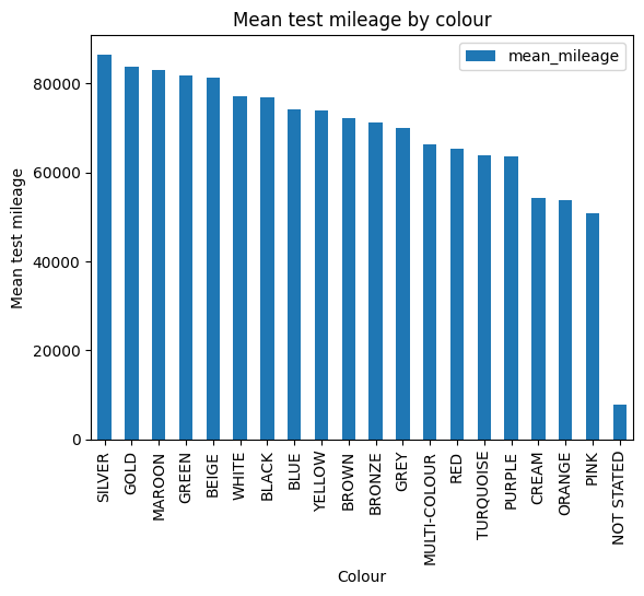
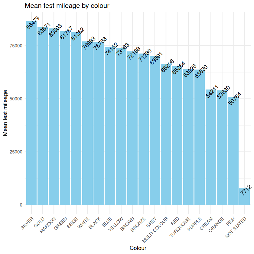
As well as calculating descriptive statistics it is important to visualize your data. Plots helps you see the spread of the data, to assess skew and to spot whether anomalies or nulls are present. In this example, we have applied mean() to show the mean test_mileage of cars grouped by colour. The argument na.rm has been added to the summarise() function which lets you decide whether you want NA values removing or leaving in the calculations. A bar chart has been used for visualisation.

PythonR

mean_mileage = (
    mot_eda_sample
    .groupby('colour')
    .agg(mean_mileage=('test_mileage','mean'))
    .sort_values(by='mean_mileage', ascending=False)
    .reset_index()
)

print(mean_mileage)

Python OutputR Output

          colour  mean_mileage
0         SILVER  86479.125043
1           GOLD  83671.474359
2         MAROON  83003.137931
3          GREEN  81787.465991
4          BEIGE  81261.990909
5          WHITE  76983.261879
6          BLACK  76787.602532
7           BLUE  74151.760425
8         YELLOW  73962.924051
9          BROWN  72189.325893
10        BRONZE  71280.473684
11          GREY  69890.805843
12  MULTI-COLOUR  66295.791667
13           RED  65283.650750
14     TURQUOISE  63925.875000
15        PURPLE  63629.895161
16         CREAM  54210.720000
17        ORANGE  53829.835664
18          PINK  50783.933333
19    NOT STATED   7712.000000

PythonR

(mean_mileage.plot(title='mean test mileage by colour', kind='bar', x='colour', y='mean_mileage')
            .set(xlabel='colour', ylabel='mean_test_mileage'))

Python OutputR Output

Further Resources

Spark at the ONS Articles:

• Big data workflow

• Sampling: an overview

• Working with duplicates