Shuffling#
This article introduces the concept of a shuffle, also referred to as an exchange. Shuffles occur when processing wide transformations such as joins and aggregations. Shuffles can be a bottleneck when processing, so it is good to understand when they occur and how to make them more efficient or minimise their use.
It covers both the theory of shuffles and practical implementations. Several topics are explored in more detail elsewhere and is recommended to read this alongside the Spark Application and UI, Partitions, Optimising Joins and Persisting articles. Some practical suggestions to improve the efficiency of shuffles include broadcast joins, salted joins and window functions.
Shuffling Concepts#
First, we will explain a few of the key concepts of shuffles, before moving on to some examples.
What is a shuffle?#
Shuffles in Spark occur when data are moved between different partitions. This is a simultaneous read and write operation and has to be fully processed before parallel processing can resume.
To fully understand this, we need to explore what we mean by partitions, and what transformations cause data to be moved between them.
What is a partition?#
Partitions are just separate chunks of data. Whereas a pandas or base R DataFrame will be stored as one object in the driver memory, a Spark DataFrame will be distributed over many different partitions on the Spark cluster. These partitions are processed in parallel wherever possible. This structure is one of the reasons that Spark is so powerful for handling large data. The Partitions article explores this topic in more detail.
In the diagram below, the solid boxes represent partitions and the arrows are transformations. If the data stays on the same partition that is referred to as as narrow transformation. Shuffles occur between the stages, where the data moves between partitions; this happens when a wide transformation is processed.
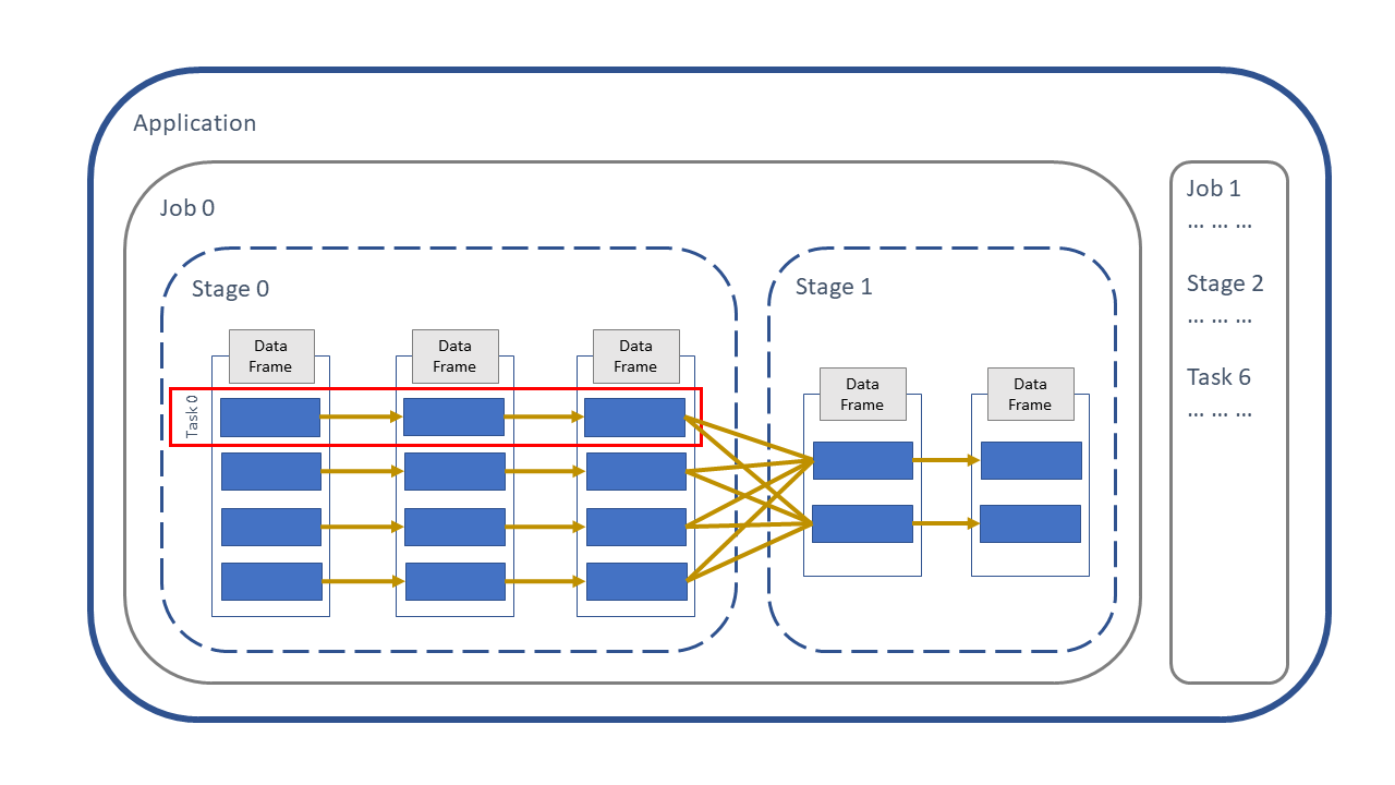
Fig. 11 Spark application#
This is covered in more detail in the Spark Application and UI article.
What transformations cause a shuffle?#
A shuffle takes place when the value of one row depends on another in a different partition, as the partitions of the DataFrame cannot then be processed in parallel. All the previous operations need to have been completed on every partition before a shuffle can take place, and then the shuffle needs to finish before anything else can happen. A good example is sorting, since the data will need to move between partitions to be in the specified order. A few examples of wide transformations:
Grouping
Aggregating
Sorting
Joining
Repartitioning
A quick note on RDDs#
Although in PySpark and sparklyr we work with DataFrames, they are actually stored in memory as a Resilient Distributed Dataset (RDD) and this is what you will see in the Spark UI.
In PySpark, a DataFrame is effectively an API built on top of the RDD, allowing it to be manipulated in a more user-friendly manner than the native RDD syntax. We can access RDD specific functionality with df.rdd; an example of this is df.rdd.getNumPartitions() to get the number of partitions of the DataFrame.
In sparklyr we simply have tbl_spark objects rather than two APIs, e.g. to get the number of partitions use sdf_num_partitions() on your sparklyr DataFrame.
From a practical perspective when coding, do not worry too much about RDDs, the concept of a shuffle works exactly the same way on a DataFrame.
Examples#
To demonstrate shuffles we will run some Spark code, and see data being transferred between partitions.
Example 1: One Shuffle#
Start with a small example to demonstrate the concept of shuffling and what actually happens to the data and partitions. First, create a Spark session. We are setting the number of partitions returned from a shuffled DataFrame to be just 2 with the spark.sql.shuffle.partitions option (the default is 200).
Note that in sparklyr with a local session spark.sql.local.partitions needs to be set; if running on a Spark cluster you can ignore this setting.
import os
from pyspark.sql import SparkSession, functions as F

spark = (
    SparkSession.builder.master("local[2]")
    .appName("shuffling")
    # Set number of partitions after a shuffle to 2
    .config("spark.sql.shuffle.partitions", 2)
    .getOrCreate()
)
library(sparklyr)
library(dplyr)

shuffle_config <- sparklyr::spark_config()
# Set number of partitions after a shuffle to 2
shuffle_config$spark.sql.shuffle.partitions <- 2
# Set number of local partitions to 2
shuffle_config$spark.sql.local.partitions <- 2

sc <- sparklyr::spark_connect(
    master = "local[2]",
    app_name = "shuffling",
    config = shuffle_config)
As we will be using random numbers in this example we set the seed, so that that repeated runs of the code will not change the results.
seed_no = 999
seed_no <- 999L
For this example, create a DataFrame with one column, id, 20 rows and two partitions using spark.range()/sdf_seq().
Now look at the DF:
example_1 = spark.range(20, numPartitions=2)
example_1.show()
example_1 <- sparklyr::sdf_seq(sc, 0, 19, repartition=2)

example_1 %>%
    sparklyr::collect() %>%
    print()
+---+
| id|
+---+
|  0|
|  1|
|  2|
|  3|
|  4|
|  5|
|  6|
|  7|
|  8|
|  9|
| 10|
| 11|
| 12|
| 13|
| 14|
| 15|
| 16|
| 17|
| 18|
| 19|
+---+
# A tibble: 20 × 1
      id
   <int>
 1     0
 2     1
 3     2
 4     3
 5     4
 6     5
 7     6
 8     7
 9     8
10     9
11    10
12    11
13    12
14    13
15    14
16    15
17    16
18    17
19    18
20    19
In order to print out the DataFrame we have to transfer the data back to the driver as one object, so we cannot see the partitioning. Indeed when we write our code we often do not pay attention to how the DataFrame might be distributed in memory.
To see how it is partitioned in Spark add another column using F.spark_partition_id()/spark_partition_id(). In PySpark this is from the functions module; in sparklyr this is Spark function called inside mutate.
example_1 = example_1.withColumn("partition_id", F.spark_partition_id())
example_1.show()
example_1 <- example_1 %>%
    sparklyr::mutate(partition_id = spark_partition_id())

example_1 %>%
    sparklyr::collect() %>%
    print()
+---+------------+
| id|partition_id|
+---+------------+
|  0|           0|
|  1|           0|
|  2|           0|
|  3|           0|
|  4|           0|
|  5|           0|
|  6|           0|
|  7|           0|
|  8|           0|
|  9|           0|
| 10|           1|
| 11|           1|
| 12|           1|
| 13|           1|
| 14|           1|
| 15|           1|
| 16|           1|
| 17|           1|
| 18|           1|
| 19|           1|
+---+------------+
# A tibble: 20 × 2
      id partition_id
   <int>        <int>
 1     0            0
 2     1            0
 3     2            0
 4     3            0
 5     4            0
 6     5            0
 7     6            0
 8     7            0
 9     8            0
10     9            0
11    10            1
12    11            1
13    12            1
14    13            1
15    14            1
16    15            1
17    16            1
18    17            1
19    18            1
20    19            1
We can see that this DataFrame has two partitions: id from 0 to 9 are in partition 0, and 10 to 19 in partition 1.
Try a transformation on this DataFrame: adding a column of random numbers, rand1, between 1 and 10 with - F.rand()/rand() and F.ceil()/ceil() (which rounds numbers up to the nearest integer), then recalculate the partition_id:
example_1 = (example_1
             .withColumn("rand1", F.ceil(F.rand(seed_no) * 10))
             .withColumn("partition_id", F.spark_partition_id()))

example_1.show()
example_1 <- example_1 %>%
    sparklyr::mutate(
        rand1 = ceil(rand(seed_no) * 10),
        partition_id = spark_partition_id())

example_1 %>%
    sparklyr::collect() %>%
    print()
+---+------------+-----+
| id|partition_id|rand1|
+---+------------+-----+
|  0|           0|    9|
|  1|           0|    4|
|  2|           0|    4|
|  3|           0|    8|
|  4|           0|    6|
|  5|           0|    2|
|  6|           0|    2|
|  7|           0|   10|
|  8|           0|    4|
|  9|           0|    3|
| 10|           1|    1|
| 11|           1|    4|
| 12|           1|    9|
| 13|           1|    6|
| 14|           1|    4|
| 15|           1|    9|
| 16|           1|    1|
| 17|           1|    6|
| 18|           1|    9|
| 19|           1|    8|
+---+------------+-----+
# A tibble: 20 × 3
      id partition_id rand1
   <int>        <int> <dbl>
 1     0            0     9
 2     1            0     4
 3     2            0     4
 4     3            0     8
 5     4            0     6
 6     5            0     2
 7     6            0     2
 8     7            0    10
 9     8            0     4
10     9            0     3
11    10            1     1
12    11            1     4
13    12            1     9
14    13            1     6
15    14            1     4
16    15            1     9
17    16            1     1
18    17            1     6
19    18            1     9
20    19            1     8
Comparing this to the previous output, we see that the partition_id has not changed. Why? This is because the data did not need to be shuffled between the partitions, as the creation of a column of random numbers is a narrow transformation. This calculation can be done independently on each row and so all partitions can be processed in parallel.
Now try sorting the data by rand1 in ascending order. Sorting will cause a shuffle, as the data needs to be moved between partitions to get it in the correct order. Then create a column for the partition_id after the sort, called partition_id_new.
example_1 = (example_1
             .orderBy("rand1")
             .withColumn("partition_id_new", F.spark_partition_id()))

example_1.show()
example_1 <- example_1 %>%
    sparklyr::sdf_sort("rand1") %>%
    sparklyr::mutate(partition_id_new = spark_partition_id())

example_1 %>%
    sparklyr::collect() %>%
    print()
+---+------------+-----+----------------+
| id|partition_id|rand1|partition_id_new|
+---+------------+-----+----------------+
| 10|           1|    1|               0|
| 16|           1|    1|               0|
|  5|           0|    2|               0|
|  6|           0|    2|               0|
|  9|           0|    3|               0|
|  1|           0|    4|               0|
|  2|           0|    4|               0|
|  8|           0|    4|               0|
| 11|           1|    4|               0|
| 14|           1|    4|               0|
|  4|           0|    6|               1|
| 13|           1|    6|               1|
| 17|           1|    6|               1|
|  3|           0|    8|               1|
| 19|           1|    8|               1|
|  0|           0|    9|               1|
| 12|           1|    9|               1|
| 15|           1|    9|               1|
| 18|           1|    9|               1|
|  7|           0|   10|               1|
+---+------------+-----+----------------+
# A tibble: 20 × 4
      id partition_id rand1 partition_id_new
   <int>        <int> <dbl>            <int>
 1    10            1     1                0
 2    16            1     1                0
 3     5            0     2                0
 4     6            0     2                0
 5     9            0     3                0
 6     1            0     4                0
 7     2            0     4                0
 8     8            0     4                0
 9    11            1     4                0
10    14            1     4                0
11     4            0     6                1
12    13            1     6                1
13    17            1     6                1
14     3            0     8                1
15    19            1     8                1
16     0            0     9                1
17    12            1     9                1
18    15            1     9                1
19    18            1     9                1
20     7            0    10                1
We can see that some data has moved between the partitions. Specifically, any row where partition_id \( \neq\) partition_id_new. Note that not all the data has changed partitions; some are already on the correct partition prior to the sorting.
As we specified spark.sql.shuffle.partitions to be 2 in the config, the shuffle has returned two partitions. In practical usage you will almost never only use two partitions, but this principle applies regardless of the size of the DF or number of partitions.
Another way to see when a shuffle has occurred is to check the Spark UI, where a shuffle is referred to as an Exchange. This is covered in more detail in the Spark Application and UI article. In a local Spark session, the URL is http://localhost:4040/.
There are different visualisations available in the Spark UI; here we will choose SQL. There should be four completed queries, which relate to the four actions we have called to this point in the Spark session.
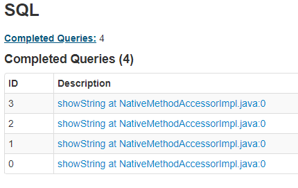
Fig. 12 Completed SQL queries#
Clicking on the link where ID is 3 displays the plan:
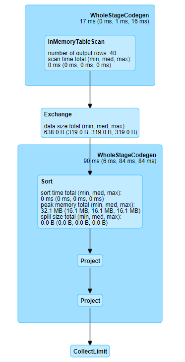
Fig. 13 Exchange in Spark UI representing a shuffle#
We can see from this that the shuffle occurred when we sorted the DataFrame by rand1, as represented by Exchange in the diagram.
Example 2: Lots of shuffles#
The previous example just had one shuffle on a tiny DF; this one has several shuffles on a larger DF, although still small by Spark standards. We will close the existing Spark session and start a new one, as the previous session had spark.sql.shuffle.partitions set to 2; here, we want 100. Be careful when closing and starting Spark sessions as existing values will be used if not explicitly defined in the new configuration.
Note that this only takes effect once we have shuffled the DataFrame, for more information on how newly created DataFrames are partitioned please refer to the Partitions article.
By default, Spark will try and use the broadcast method for joins. We want to ensure that we demonstrate the behaviour of the regular join (sort merge join) and so are deactivating automatic broadcast joins in the configuration by setting spark.sql.autoBroadcastJoinThreshold to -1.
spark.stop()

spark = (
    SparkSession.builder.master("local[2]")
    .appName("shuffling")
    # Set number of partitions after a shuffle to 100
    .config("spark.sql.shuffle.partitions", 100)
    # Disable broadcast join by default
    .config("spark.sql.autoBroadcastJoinThreshold", -1)
    .getOrCreate()
)
sparklyr::spark_disconnect(sc)

shuffle_config <- sparklyr::spark_config()
# Set number of partitions after a shuffle to 100
shuffle_config$spark.sql.shuffle.partitions <- 100
# Set number of local partitions to 100
shuffle_config$spark.sql.local.partitions <- 100
# Disable broadcast join by default
shuffle_config$spark.sql.autoBroadcastJoinThreshold <- -1

sc <- sparklyr::spark_connect(
    master = "local[2]",
    app_name = "shuffling",
    config = shuffle_config)
Here we create two DataFrames of \(100,000\) rows and add a random number between 1 to 10 for each called rand1 and rand2 respectively, using the same method as previously.
# Create two DataFrames
example_2A = spark.range(10**5).withColumn("rand1", F.ceil(F.rand(seed_no) * 10))
example_2B = spark.range(10**5).withColumn("rand2", F.ceil(F.rand(seed_no + 1) * 10))
example_2A <- sparklyr::sdf_seq(sc, 0, 10**5 - 1) %>%
    sparklyr::mutate(rand1 = ceil(rand(seed_no) * 10))

example_2B <- sparklyr::sdf_seq(sc, 0, 10**5 - 1) %>%
    sparklyr::mutate(rand2 = ceil(rand(seed_no + 1L) * 10))
We now want to perform some transformations which involve a shuffle. Let’s create a new DataFrame, joined_df, by joining example_2B to example_2A. We then group by rand1 and rand2, then sort by rand1 and rand2.
joined_df = (example_2A.
             join(example_2B, on="id", how="left")
             .groupBy("rand1", "rand2")
             .agg(F.count(F.col("id")).alias("row_count"))
             .orderBy("rand1", "rand2"))
joined_df <- example_2A %>%
    sparklyr::left_join(example_2B, by="id") %>%
    dplyr::group_by(rand1, rand2) %>%
    dplyr::summarise(row_count = n()) %>%
    sparklyr::sdf_sort(c("rand1", "rand2"))
For the action, we are calling a collect-style operation (.toPandas()/collect()) rather than .show(n) (PySpark) or head(n) %>% collect() (sparklyr). The reason is .show(n)/head(n) will only do the minimum required to return n rows, whereas .toPandas()/collect() causes all the data to be collected to the driver from the Spark cluster, forcing a full calculation.
Then sanity check the result, by getting the row count and the top and bottom 5 rows:
collected_df = joined_df.toPandas()

print("Row count: ", collected_df.shape[0])
print("\nTop 5 rows:\n", collected_df.head(5))
print("\nBottom 5 rows:\n", collected_df.tail(5))
collected_df <- joined_df %>%
    sparklyr::collect()

print("Row count: ")
print(nrow(collected_df))
print("Top 5 rows:")
print(head(collected_df, 5))
print("Bottom 5 rows:")
print(tail(collected_df, 5))
Row count:  100

Top 5 rows:
    rand1  rand2  row_count
0      1      1        969
1      1      2        988
2      1      3       1023
3      1      4       1033
4      1      5        976

Bottom 5 rows:
     rand1  rand2  row_count
95     10      6        963
96     10      7       1004
97     10      8       1023
98     10      9        989
99     10     10        959
[1] "Row count: "
[1] 100
[1] "Top 5 rows:"
# A tibble: 5 × 3
  rand1 rand2 row_count
  <dbl> <dbl>     <dbl>
1     1     1       969
2     1     2       988
3     1     3      1023
4     1     4      1033
5     1     5       976
[1] "Bottom 5 rows:"
# A tibble: 5 × 3
  rand1 rand2 row_count
  <dbl> <dbl>     <dbl>
1    10     6       963
2    10     7      1004
3    10     8      1023
4    10     9       989
5    10    10       959
The result is as expected.
Rather than try and print out the partition_id like we did in the first example, here the Spark UI is much more informative:
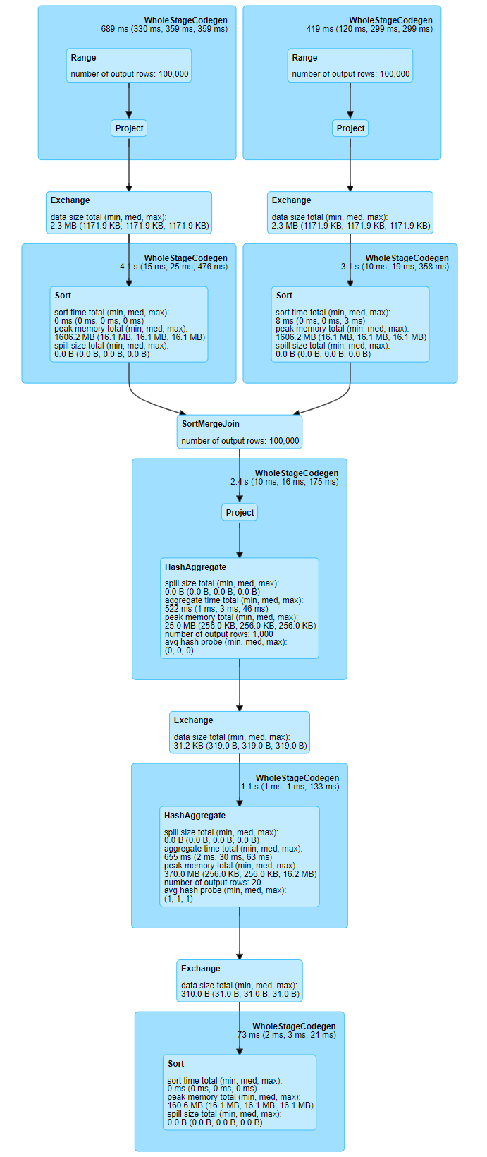
Fig. 14 Multiple exchanges#
We can visually see where a shuffle takes place, in this case, on both DataFrames prior to the join, then when grouping, and finally one more when sorting at the end.
A quick note on the shuffles prior to the join: Spark uses sort merge join, which requires a shuffle of the DataFrames before performing the join, hence the initial Exchange and Sort in the diagram. The other joining algorithm is the broadcast join, briefly covered later and in full in the Join Concepts article.
Optimising and Avoiding Shuffles#
Now we have seen some examples of shuffles, let us explain properly why we generally want to minimise unnecessary use of them.
The shuffle itself is an expensive operation, by which we mean it takes a long time to run compared to most other operations. In addition, when the data are being shuffled, all prior operations have to complete first. This is why the steps in the Spark UI are referred to as stages; all the processing in one stage has to be completed before the next one can start.
As such shuffles can cause bottlenecks in our code and slow it down.
It is very unlikely that you will be able to avoid using shuffles completely. Grouping, aggregations, joining and ordering are almost essential when writing Spark codes. So the important thing is to understand shuffles and use them sensibly, rather than being afraid of them!
Minimise actions and caching#
Remember how Spark works: it is a set of transformations, which are triggered by an action. The action will process the entire Spark plan. You could have written your code very efficiently to minimise the number of shuffles, but if you are calling repeated actions then these shuffles will also be repeated.
During development you may have actions to preview the data (e.g. .show()/glimpse()) or to get the row count (.count()/sdf_nrow()) at interim parts of the code, to understand how your DataFrame is changing and to help debug the code. Before repeatedly running analysis or releasing production code you will want to eliminate any of these superfluous actions.
You can make careful use of persisting in these situations, such as caching, checkpointing or using staging tables; see the persisting article for more detail.
In addition, Spark does have some efficiencies in the way repeated actions are handled but in general, try and minimise the number of actions that you call if they are not needed.
Converting to pandas or base R DF#
If your DataFrame is small, you can discard the concept of distributed computing and shuffling entirely by converting it into a pandas or base R DataFrame and process it in the driver memory rather than in Spark. Operations which would normally trigger a shuffle in Spark will be instead processed in the driver memory.
Converting PySpark DataFrames to pandas is very easy as they have a .toPandas() method. In sparklyr, use sparklyr::collect(); this will convert to the standard dplyr-style tibble, which are mostly interchangeable with base R DFs.
In PySpark you can even skip Spark entirely by reading in from HDFS to pandas with Pydoop.
Be careful; if your DF is large, there may not be enough driver memory to process it and you will get an error. Choosing between Spark and pandas/base R is something that should be done at the start of a project and should be carefully considered; if you choose to use the driver memory and find that there is insufficient capacity then you will have to re-write your code in Spark, which is often not a trivial task. See the When To Use Spark article for more information.
Reduce size of DataFrame#
The larger the DataFrame that is supplied to Spark the longer the Spark job will take. If it is possible to reduce the size of the DataFrame then most operations on the DF should be more efficient, including shuffling. An example could be moving a filter operation to earlier in the code. Note that Spark does have some optimisation in terms of orders of operations, but where possible try and work with smaller DFs if possible.
Use a broadcast join#
As we saw in the second example, a join will cause a shuffle on the DataFrames to be joined. We saw that this was referred to as a SortMergeJoin in the visualised plan. There is however another type of join: the broadcast join. A broadcast join can be used when one of your DataFrames in the join is small; a copy is created on each partition. This can then be processed separately on each partition in parallel, avoiding the need for a full shuffle.
Broadcast joins are one of the easiest ways to improve the efficiency of your code, as you just have to wrap the second DF in F.broadcast() in PySpark or sdf_broadcast()
in sparklyr.
The Optimising Joins article has full details; this is an example of the Spark UI from that article, showing that there are fewer shuffles involved when broadcasting:
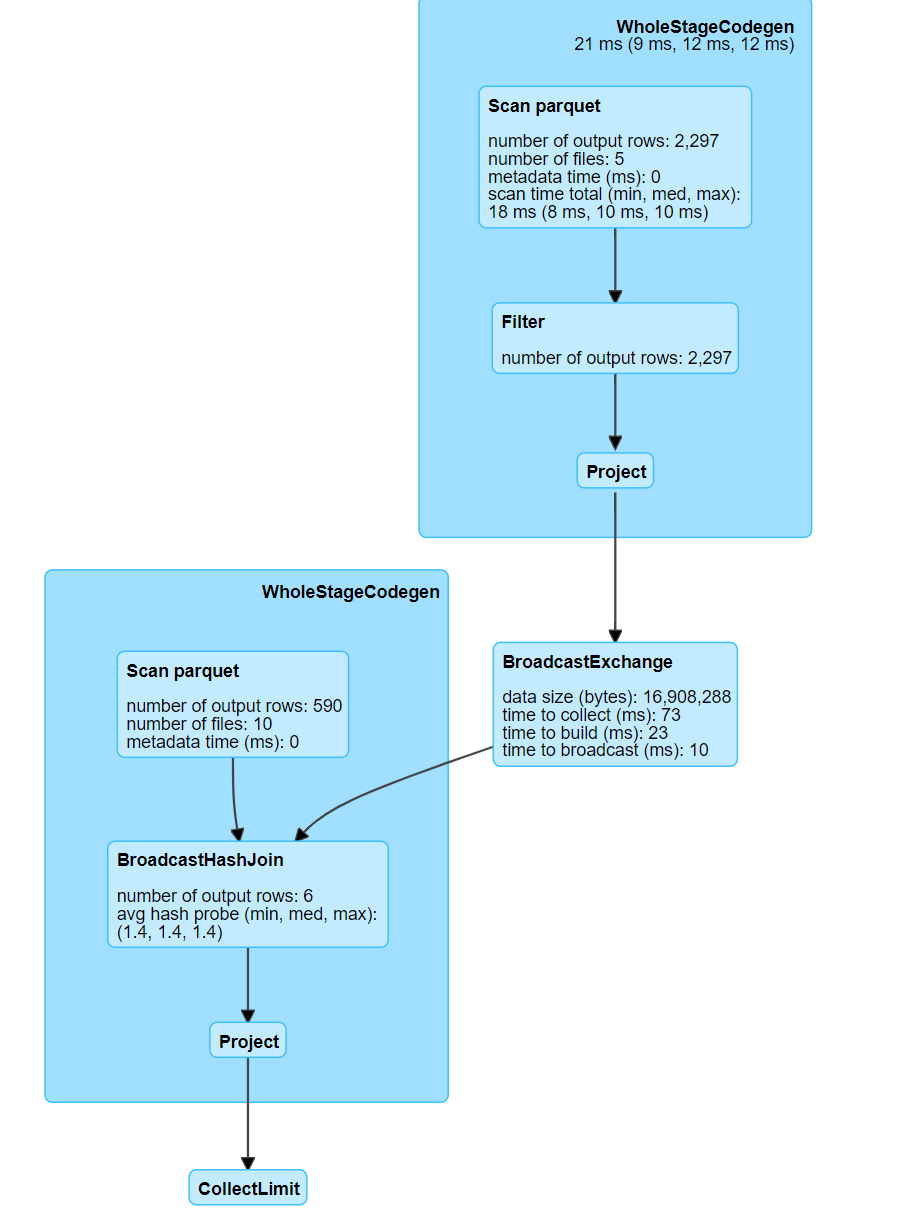
Fig. 15 Boradcast exchange#
Replace joins with conditional statements#
If you are joining a tiny DataFrame of only a few rows, a shuffle can potentially be avoided entirely be re-writing the join as a set of conditional statements with F.when() in PySpark or case_when()
in sparklyr; although this method can be more prone to errors when coding and harder to maintain. See the Optimising Joins: Replacing a join with a narrow transformation section for more information.
Avoiding unnecessary sorting#
There can be the temptation to put a lot of .orderBy()/sdf_sort() statements in your code when developing, especially if you are previewing the data at various points (e.g. with show(n)/head(n) %>% collect()). Remember that our Spark DataFrames are distributed into partitions and so the concept of order is different to when we have these stored as one object (e.g. a pandas or R DataFrame) in the driver memory. Generally the order of the rows in the DataFrame should not matter; you can often just sort the data once right at the end of the code before writing out the results if the order of the output is important.
This does come with a caveat in that Spark sometimes can be cleverer than we expect, due to the catalyst optimizer. As we know, the Spark plan is only triggered when an action is called, such as .show(), collect() etc. Spark will sometimes however detect unnecessary sorting and optimise the plan. We can demonstrate this by sorting our DataFrame several times, then looking at the UI.
In sparklyr, sdf_sort() can only sort ascending, so a temporary column of negative values is created, then dropped at the end. arrange() can sort descending, although this is only triggered if collected immediately or used in conjunction with head().
Note that the code below is being re-assigned on each line rather than being chained; this is to demonstrate that it is not the chaining which causes Spark to optimise the code.
unsorted_df = spark.range(10 ** 5).withColumn("rand1", F.ceil(F.rand(seed_no) * 10))

sorted_df = unsorted_df.orderBy("rand1", ascending=True)
sorted_df = sorted_df.orderBy("rand1", ascending=False)
sorted_df = sorted_df.orderBy("rand1", ascending=True)
sorted_df = sorted_df.orderBy("rand1", ascending=False)
sorted_collected_df = sorted_df.toPandas()

print("Row count: ", sorted_collected_df.shape[0])
print("\nTop 5 rows:\n", sorted_collected_df.head(5))
print("\nBottom 5 rows:\n", sorted_collected_df.tail(5))
unsorted_df <- sparklyr::sdf_seq(sc, 0, 10**5 - 1) %>%
    sparklyr::mutate(rand1 = ceil(rand(seed_no) * 10),
                     # Create temporary column for sorting descending
                     rand2 = rand1 * -1)

sorted_df <- unsorted_df %>% sparklyr::sdf_sort("rand1")
sorted_df <- sorted_df %>% sparklyr::sdf_sort("rand2")
sorted_df <- sorted_df %>% sparklyr::sdf_sort("rand1")
sorted_df <- sorted_df %>% sparklyr::sdf_sort("rand2") %>%
    # Remove temporary column used to sort descending
    sparklyr::select(-rand2)

sorted_collected_df <- sorted_df %>%
    sparklyr::collect()

print("Row count: ")
print(nrow(sorted_collected_df))
print("Top 5 rows:")
print(head(sorted_collected_df, 5))
print("Bottom 5 rows:")
print(tail(sorted_collected_df, 5))
Row count:  100000

Top 5 rows:
    id  rand1
0   7     10
1  19     10
2  21     10
3  24     10
4  58     10

Bottom 5 rows:
           id  rand1
99995  99930      1
99996  99936      1
99997  99947      1
99998  99963      1
99999  99975      1
[1] "Row count: "
[1] 100000
[1] "Top 5 rows:"
# A tibble: 5 × 2
     id rand1
  <int> <dbl>
1     7    10
2    19    10
3    21    10
4    24    10
5    58    10
[1] "Bottom 5 rows:"
# A tibble: 5 × 2
     id rand1
  <int> <dbl>
1 99930     1
2 99936     1
3 99947     1
4 99963     1
5 99975     1
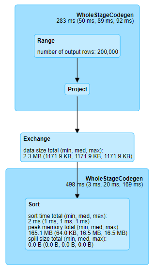
Fig. 16 Multiple sorts in single exchange#
On the plan, we only have one exchange, but we gave it four operations which should cause a shuffle. What has happened is that Spark has optimised the plan to only include one shuffle. This is a feature of Spark called the catalyst optimizer and is explained further in the Persisting article.
We can demonstrate this by looking at the full plan with .explain(True)
in PySpark and with invoke("queryExecution") in sparklyr:
sorted_df.explain(True)
sorted_df %>%
    sparklyr::spark_dataframe() %>%
    sparklyr::invoke("queryExecution")
== Parsed Logical Plan ==
'Sort ['rand1 DESC NULLS LAST], true
+- Sort [rand1#77L ASC NULLS FIRST], true
   +- Sort [rand1#77L DESC NULLS LAST], true
      +- Sort [rand1#77L ASC NULLS FIRST], true
         +- Project [id#75L, CEIL((rand(999) * cast(10 as double))) AS rand1#77L]
            +- Range (0, 100000, step=1, splits=Some(2))

== Analyzed Logical Plan ==
id: bigint, rand1: bigint
Sort [rand1#77L DESC NULLS LAST], true
+- Sort [rand1#77L ASC NULLS FIRST], true
   +- Sort [rand1#77L DESC NULLS LAST], true
      +- Sort [rand1#77L ASC NULLS FIRST], true
         +- Project [id#75L, CEIL((rand(999) * cast(10 as double))) AS rand1#77L]
            +- Range (0, 100000, step=1, splits=Some(2))

== Optimized Logical Plan ==
Sort [rand1#77L DESC NULLS LAST], true
+- Project [id#75L, CEIL((rand(999) * 10.0)) AS rand1#77L]
   +- Range (0, 100000, step=1, splits=Some(2))

== Physical Plan ==
*(2) Sort [rand1#77L DESC NULLS LAST], true, 0
+- Exchange rangepartitioning(rand1#77L DESC NULLS LAST, 100)
   +- *(1) Project [id#75L, CEIL((rand(999) * 10.0)) AS rand1#77L]
      +- *(1) Range (0, 100000, step=1, splits=2)
<jobj[73]>
  org.apache.spark.sql.execution.QueryExecution
  == Parsed Logical Plan ==
'Project ['id, 'rand1]
+- 'UnresolvedRelation `sparklyr_tmp_84a4a495_8926_4508_a776_58e5d785612b`

== Analyzed Logical Plan ==
id: int, rand1: bigint
Project [id#67, rand1#75L]
+- SubqueryAlias `sparklyr_tmp_84a4a495_8926_4508_a776_58e5d785612b`
   +- Sort [rand2#76 ASC NULLS FIRST], true
      +- Project [id#67, rand1#75L, rand2#76]
         +- SubqueryAlias `sparklyr_tmp_4bead31f_cb75_477e_9a7a_fe93cc69940a`
            +- Sort [rand1#75L ASC NULLS FIRST], true
               +- Project [id#67, rand1#75L, rand2#76]
                  +- SubqueryAlias `sparklyr_tmp_69f825f8_040d_45cf_b014_5213f38e0dd8`
                     +- Sort [rand2#76 ASC NULLS FIRST], true
                        +- Project [id#67, rand1#75L, rand2#76]
                           +- SubqueryAlias `sparklyr_tmp_245f1eba_188c_4a73_b9de_cf51ad1bd30d`
                              +- Sort [rand1#75L ASC NULLS FIRST], true
                                 +- Project [id#67, rand1#75L, CheckOverflow((promote_precision(cast(cast(rand1#75L as decimal(20,0)) as decimal(21,1))) * promote_precision(cast(-1.0 as decimal(21,1)))), DecimalType(23,1)) AS rand2#76]
                                    +- SubqueryAlias `q01`
                                       +- Project [id#67, CEIL((rand(999) * cast(10.0 as double))) AS rand1#75L]
                                          +- SubqueryAlias `sparklyr_tmp_e3c999d4_6b13_4147_b556_e71bf666f08f`
                                             +- LogicalRDD [id#67], false

== Optimized Logical Plan ==
Project [id#67, rand1#75L]
+- Sort [rand2#76 ASC NULLS FIRST], true
   +- Project [id#67, rand1#75L, CheckOverflow((promote_precision(cast(cast(rand1#75L as decimal(20,0)) as decimal(21,1))) * -1.0), DecimalType(23,1)) AS rand2#76]
      +- Project [id#67, CEIL((rand(999) * 10.0)) AS rand1#75L]
         +- LogicalRDD [id#67], false

== Physical Plan ==
*(2) Project [id#67, rand1#75L]
+- *(2) Sort [rand2#76 ASC NULLS FIRST], true, 0
   +- Exchange rangepartitioning(rand2#76 ASC NULLS FIRST, 100)
      +- *(1) Project [id#67, rand1#75L, CheckOverflow((promote_precision(cast(cast(rand1#75L as decimal(20,0)) as decimal(21,1))) * -1.0), DecimalType(23,1)) AS rand2#76]
         +- *(1) Project [id#67, CEIL((rand(999) * 10.0)) AS rand1#75L]
            +- Scan ExistingRDD[id#67]
The key output here is the difference between the Parsed and Analyzed Logical Plans, and the Optimized Logical Plan. We can see in the first two that all our sorting operations are present, but in the Optimized, only the final sort is. Hence we only have one shuffle.
Use Window functions#
One way to reduce the number of shuffles is to ensure that you are using window functions where possible. One example is deriving a new column which depends on the total of a group. One way is to create a new DataFrame with the group totals, then join that back to the original DataFrame, then use this in the calculation. This will involve shuffles for the grouping/aggregation and the join, whereas a window function will only need one.
Another benefit is that the code is neater and easier to read with a window function. See the article on Window Functions for more information.
Other things matter too!#
A final word on avoiding shuffles: do not let this distract you from everything else that you need to consider when writing good code! While it is important to understand shuffles and to try and implement the methods above where you can, it is better to have code which works, then optimise it afterwards. Also remember that with code there is a never a final version: provided it is well written, appropriately commented and has good unit tests, you or a colleague can always re-visit it to optimise it at a later date.
Some shuffles can actually be relatively quick, depending on factors including the total size of the DataFrame, the number of partitions, and how it is partitioned. It can be worth checking the Spark UI to see exactly how much time your shuffle is taking.
Although removing or optimising shuffles is one of the most obvious ways to improve the efficiency of your code, when looking at ways to improve the performance of your code make sure you look at other elements too.
Good Shuffles#
We’ve seen how shuffles take time to process and can cause a bottleneck in performance. However, this is not always the case.
Sometimes shuffling our data into more logical partitions can actually cause performance to increase. For instance, if our data are skewed so that one partition contains significantly more data than another, the parallelism will not be as efficient as it could be. By shuffling the data into partitions of similar sizes, the efficiency will actually increase. An example is using a salted join to reduce skew when joining DataFrames.
You can also change the number of partitions. By default, this is 200, but repartitioning into a greater or smaller number depending on your data and what you are doing with it can help performance. Note that when repartitioning a DataFrame, .repartition()/sdf_repartition() will cause a full shuffle into roughly equal partition sizes, whereas .coalesce()/sdf_coalesce() will essentially combine partitions (and so they may vary in size), so the data will still move but be processed more efficiently. This topic is explored more in the Partitions article.
Summary#
In this article we have demonstrated:
What a shuffle is and why they are essential in a distributed environment
When they occur
Why they can be a bottleneck on performance
How to optimise and minimise them in your code
Why they can sometimes be beneficial
Further Resources#
Spark at the ONS Articles:
-
Broadcast Join
Sort Merge Join
Replacing a join with a narrow transformation
PySpark Documentation:
sparklyr and tidyverse Documentation:
Spark SQL Documentation:
Spark documentation:
Performance tuning: details of
spark.sql.shuffle.partitionsandspark.sql.autoBroadcastJoinThreshold
Other Links: