Managing Partitions

DataFrames in Spark are distributed, so although we treat them as one object they might be split up into multiple partitions over many machines on the cluster. The benefit of having multiple partitions is that some operations can be performed on the partitions in parallel.

More partitions means greater parallelisation. However, there is a cost associated with multiple partitions, for example scheduling delay and data serialisation. In the Spark Application and UI article we saw that putting a small DataFrame into one or two partitions can lead to more efficient processing.

In this notebook we will explore these partitions and how the partitioning of a DataFrame is affected by importing, processing and writing data in Spark. The goal is not to find the optimum number of partitions for a given DataFrame, the goal is to have greater awareness of partitioning so we can avoid the extreme cases of over-partitioning, under-partitioning and highly skewed partitioning.

Investigating partitions

We will start by investigating the partitions of some DataFrames. We will look at the partitions of a newly created DataFrame, an imported DataFrame and a processed DataFrame. But first, we’ll need to do some imports and create a local application in the usual way.

PythonR

import yaml
from pyspark.sql import SparkSession, Window, functions as F

spark = (SparkSession.builder.master("local[2]")
         .appName("partitions")
         .getOrCreate())

Newly created DataFrame

Let’s create a DataFrame called rand_df with an id column from 0 to 4,999 and a rand_val column containing random numbers from 1 to 10.

PythonR

row_ct = 5000
seed_no = 42 #this is used to create the pseudo-random numbers

rand_df = spark.range(0, row_ct)
rand_df = rand_df.withColumn("rand_val", F.ceil(F.rand(seed=seed_no)*10))

rand_df.show(10)

Python OutputR Output

+---+--------+
| id|rand_val|
+---+--------+
|  0|       7|
|  1|       9|
|  2|      10|
|  3|       9|
|  4|       5|
|  5|       6|
|  6|       1|
|  7|       2|
|  8|       4|
|  9|       7|
+---+--------+
only showing top 10 rows

To find the number of partitions of a DataFrame in PySpark we need to access the underlying RDD structures that make up the DataFrame by using .rdd after referencing the DataFrame. Then we can use the .getNumPartitions() method to return the number of partitions. In sparklyr we can just use the function sdf_num_partitions().

We can also find out how many rows are in each partition. There is more than one way of doing this, one method was introduced in the Shuffling article and will be used later in this article, a second method is shown below. Again, in PySpark we will need to access the underlying RDDs then map on a lambda function that will loop over the rows in each partition and return a count of these rows in a list. In sparklyr we can use spark_apply() to give us a row count for each partition.

Don’t worry too much about understanding this line of code, it’s the result which is important here.

PythonR

print('Number of partitions:\t\t', rand_df.rdd.getNumPartitions())

rows_in_part = rand_df.rdd.mapPartitions(lambda x: [sum(1 for _ in x)]).collect()
print('Number of rows per partition:\t', rows_in_part)

Python OutputR Output

Number of partitions:		 2
Number of rows per partition:	 [2500, 2500]

Note that the size of the partitions is the same. We will see later, if there was skew in partition sizes we would always have to wait for the largest partition to finish processing before moving on to the next task, this is commonly referred to as a bottleneck. So Spark understandably puts a similar number of rows in each partition.

The number of partitions was set by default. The property that controls this number is spark.default.parallelism, and to modify the default we must override it in the Spark session. See the Guidance on Spark Sessions for more information on how to do this. To see what the default is we can look at the Spark documentation (if you follow the link use Ctrl+F to search for the property name).

For operations like parallelize with no parent RDDs, it depends on the cluster manager:

• Local mode: number of cores on the local machine

• Mesos fine grained mode: 8

• Others: total number of cores on all executor nodes or 2, whichever is larger

We’re running Spark in local mode with 2 cores, hence without overriding this property it will default to 2.

Modifying the spark.default.parallelism property will set the number of partitions for all newly created DataFrames in this session. But what if we want to create a DataFrame that is unusually large or small for our session? For this case we can specify how many partitions we want when creating the DataFrame, using an extra argument numPartitions/repartition for PySpark/sparklyr.

PythonR

small_rand = spark.range(0, 10, numPartitions=1) #just 10 rows, so we'll put them into one partition
small_rand = small_rand.withColumn("rand_value",  F.ceil(F.rand(seed=seed_no)*10))

small_rand.show()
small_rand.rdd.getNumPartitions()

Python OutputR Output

+---+----------+
| id|rand_value|
+---+----------+
|  0|         7|
|  1|         9|
|  2|        10|
|  3|         9|
|  4|         5|
|  5|         6|
|  6|         1|
|  7|         2|
|  8|         4|
|  9|         7|
+---+----------+
1

Imported DataFrame

Next, let’s import the animal_rescue.csv file and see how many partitions we have.

PythonR

with open("../../../config.yaml") as f:
    config = yaml.safe_load(f)
    
rescue_path = config["rescue_path_csv"]

rescue = spark.read.csv(rescue_path, header=True, inferSchema=True)

rescue.rdd.getNumPartitions()

Python OutputR Output

1

Again, we didn’t set this number anywhere, and it obviously wasn’t set by spark.default.parallelism either.

How many rows and columns do each DataFrame have?

PythonR

rescue_rows = rescue.count()
rescue_columns = len(rescue.columns)

rand_df_columns = len(rand_df.columns)

print('Number of rows in rescue DataFrame:\t\t', rescue_rows)
print('Number of columns in rescue DataFrame:\t\t', rescue_columns)
print('Total number of cells in rescue DataFrame:\t', rescue_rows*rescue_columns)
print('\nNumber of rows in random_df DataFrame:\t\t', row_ct)
print('Number of columns in random_df DataFrame:\t', rand_df_columns)
print('Total number of cells in random_df DataFrame:\t', len(rand_df.columns)*row_ct)

Python OutputR Output

Number of rows in rescue DataFrame:		 5898
Number of columns in rescue DataFrame:		 26
Total number of cells in rescue DataFrame:	 153348

Number of rows in random_df DataFrame:		 5000
Number of columns in random_df DataFrame:	 2
Total number of cells in random_df DataFrame:	 10000

There are more cells in the rescue DataFrame, but Spark put it into just one partition.

The reason for this is that the original csv file is stored as a single file on disk, which means that Spark will read it in as one partition. Data on HDFS can be stored in multiple files. In general, when a Spark DataFrame with \(P\) partitions is written onto disk, it will be stored in \(P\) files, and whenever we read that dataset into a Spark session it will again have \(P\) partitions. We will revisit writing partitions to disk later.

Processed DataFrame

Let’s see how applying narrow and wide transformations to the DataFrame affects the number of partitions. Firstly we’ll filter the data, which is a narrow operation.

PythonR

filtered_rescue = rescue.filter(F.col('AnimalGroupParent') == 'Cat')
filtered_rescue.select('AnimalGroupParent', 'FinalDescription').show(3, truncate=False)

print('Number of partitions in filtered_rescue DataFrame:\t',filtered_rescue.rdd.getNumPartitions())

Python OutputR Output

+-----------------+--------------------------------------------+
|AnimalGroupParent|FinalDescription                            |
+-----------------+--------------------------------------------+
|Cat              |TO ASSIST RSPCA WITH CAT TRAPPED UP TREE,B15|
|Cat              |ASSIST RSPCA WITH CAT STUCK UP TREE, B15    |
|Cat              |CAT STUCK UP TREE,B15                       |
+-----------------+--------------------------------------------+
only showing top 3 rows

Number of partitions in filtered_rescue DataFrame:	 1

No change. In general, for a narrow transformations the contents of the partitions will change according to the transformation applied, but no data will move from one partition to another and the total number of partitions will remain the same.

Now let’s group the data, which is a wide operation, by PostcodeDistrict and then aggregate to find a count of incidents by area. How many partitions will we have in the new DataFrame?

*Note PySpark and sparklyr will give different results here; we will explain why later.

PythonR

count_by_area = (rescue.groupBy('PostcodeDistrict')
    .agg(F.count('IncidentNumber').alias('Count')))

count_by_area.show(5)
print('Number of partitions in rescue_by_area DataFrame:\t', count_by_area.rdd.getNumPartitions())

Python OutputR Output

+----------------+-----+
|PostcodeDistrict|Count|
+----------------+-----+
|            SE17|   20|
|            EC1Y|    1|
|             CR0|   98|
|             EN3|   45|
|            SW14|   12|
+----------------+-----+
only showing top 5 rows

Number of partitions in rescue_by_area DataFrame:	 200

How many?!?

😵

Let’s check how many rows are in each partition.

PythonR

rows_in_part = count_by_area.rdd.mapPartitions(lambda x: [sum(1 for _ in x)]).collect()
print('Number of rows per partition:\t', rows_in_part)

Python OutputR Output

Number of rows per partition:	 [1, 1, 1, 0, 0, 0, 1, 1, 2, 1, 2, 1, 0, 1, 1, 0, 1, 2, 2, 4, 1, 2, 1, 0, 2, 3, 2, 3, 1, 2, 0, 1, 1, 3, 0, 0, 2, 3, 0, 1, 1, 2, 1, 1, 3, 0, 2, 2, 1, 2, 1, 2, 0, 3, 5, 4, 1, 1, 1, 2, 0, 2, 2, 1, 0, 1, 1, 0, 0, 0, 1, 1, 4, 3, 1, 2, 3, 3, 1, 4, 0, 2, 2, 5, 1, 1, 0, 0, 3, 1, 3, 2, 1, 1, 0, 1, 1, 1, 1, 1, 1, 1, 2, 3, 3, 0, 2, 0, 1, 2, 2, 0, 1, 6, 0, 2, 0, 1, 1, 1, 1, 0, 1, 1, 0, 0, 2, 2, 1, 3, 1, 3, 1, 3, 0, 0, 1, 4, 1, 4, 1, 0, 0, 0, 1, 1, 3, 1, 2, 3, 1, 0, 1, 0, 2, 1, 1, 2, 1, 0, 2, 1, 1, 1, 1, 1, 1, 1, 0, 1, 0, 1, 2, 4, 2, 0, 1, 0, 0, 1, 2, 3, 2, 1, 0, 1, 0, 3, 2, 0, 2, 1, 0, 4, 0, 2, 0, 0, 0, 3]

Quite a few empty partitions- this is a clear case of overpartitioning. In the Spark Application and UI article it was shown that overpartitioning leads to slower processing as a larger proportion of time is spent on scheduling tasks and (de)serialising data instead of processing the task.

Again, there is a property we can modify in the Spark session configuration to change this behaviour. The property to override is spark.sql.shuffle.partitions. Shuffle partitions means when a shuffle occurs, for example a wide operation. So this property says “give the resulting DataFrame this many partitions”. See the article on Shuffling for more information on shuffles.

The Spark documentation shows that the default value for spark.sql.shuffle.partitions is 200. This default is obviously too high for our case of grouping a small dataset with a small number of groups i.e. PostcodeDistrict. This is one of the more useful properties to consider changing depending on the size of the data you want to process with Spark.

We noted above that sparklyr would give different results. Using a local sparklyr session there is another property that is used for partitioning after a wide operation, spark.sql.shuffle.partitions.local, which is set to 16 by default.

How to change partitioning

Before we look at how to modify DataFrame partitioning, let’s revisit the motivation for wanting to do this.

Motivation

1. We can change the number of partitions of a DataFrame to achieve less or more parallelisation. More parallel processing is great for large DataFrames, but there are some scheduling and data serialisation overheads involved in processing multiple partitions. So for small DataFrames it’s best to have just a small number of partition because the overheads involved in organising and writing multiple partitions will result in slower processing. However, we don’t always get to choose the partitioning, e.g. to do a join Spark must first put rows with the same join keys on the same partition. More on this later.

2. We can also partition by a specified column(s) in the DataFrame. This can be useful when writing to a Hive table or file becuase we can then read in single partitions. For example, say we had a DataFrame containing records from the past 20 years. We could partition this DataFrame by year when writing it to disk, then in future we could read in one year at a time or multiple years to speed up future tasks.

Change partitioning

Here are two ways of changing the number of partitions of a DataFrame. One is .repartition()/sdf_repartition() and the other is coalesce()/sdf_coalesce().

Let’s see how to use these functions.

PythonR

rand_df.rdd.getNumPartitions()

Python OutputR Output

2

PythonR

rand_df = rand_df.coalesce(1)
rand_df.rdd.getNumPartitions()

Python OutputR Output

1

PythonR

rand_df = rand_df.coalesce(10)
rand_df.rdd.getNumPartitions()

Python OutputR Output

2

Is that the answer we were expecting? Note that .coalesce() should only be used to decrease the number of partitions. When increasing it can only increase to a previous state.

PythonR

rand_df = rand_df.repartition(1)
rand_df.rdd.getNumPartitions()

Python OutputR Output

1

PythonR

rand_df = rand_df.repartition(10)
rand_df.rdd.getNumPartitions()

Python OutputR Output

10

Repartition can be used to increase parallelisation.

The other important difference is that .repartition() incurs a full shuffle of the DataFrame, meaning it rewrites all the data into the new partitions. Shuffling takes time, especially for large amounts of data, so it’s best to avoid shuffling more data than needed. To learn more about shuffling have a look at the Shuffling article.

On the other hand .coalesce() involves moving just some of the data. Let’s demonstrate by an example.

Say we have a simple DataFrame where the partitions contain the following numbers:

Partition 1: 1, 2, 3
Partition 2: 4, 5, 6
Partition 3: 7, 8, 9
Partition 4: 10, 11, 12

We then decide we want two partitions as opposed to four so we apply .coalesce(2) to the DataFrame. The partitions would now contain the following:

Partition 1: 1, 2, 3 + (7, 8, 9)
Partition 2: 4, 5, 6 + (10, 11, 12)

So the data on Partitions 1 and 2 have not been shuffled. We have just moved the data on Partitions 3 to Partition 1 and Partition 4 to Partition 2, this is sometimes referred to as a partial shuffle. The gains from this simple example would be negligible, but scale this process up to millions of rows and then it becomes significant.

It’s also possible to use a column name in .repartition() or even a number and column name, see documentation for more information.

Partition sizes

A key concept in both Hadoop and Spark is that files and partitions should optimally be around 128MB. It is however common that data are stored as many small files rather than fewer large ones. This issue can be solved by reducing the number of partitions before writing to HDFS, using .coalesce() or .repartition() in PySpark and sdf_coalesce() or sdf_repartition() in sparklyr.

Below are two reasons why it’s a good idea to avoid writing out many small files.

Avoiding the small files issue on HDFS

HDFS consists of many DataNodes, which store the files, and a single NameNode, which essentially works as an index for the file system. The small files issue occurs as every file path is loaded into the NameNode which leads to an inefficient use of the memory capacity, e.g. if a 600MB file is stored as 200 files of 3MB then the NameNode needs to load 200 file paths, instead of the 5 file paths it would have to load if stored as 5 files of 120MB each.

More efficient processing with Spark

Spark will by default use one partition per file on disk when reading in the data. If there are many small files on disk then these will be converted to many small partitions, which leads to slower processing as proportionally more time is spent scheduling tasks and serialising data.

Intermediate partitions in wide operations

Now onto a more complex topic of intermediate partitioining.

We saw earlier that for narrow transformations the number of partitions of input and output DataFrames is the same. We also saw that for wide transformations the number of partitions of the output DataFrame is changed to the value of the spark.sql.shuffle.partitions property set in the Spark session.

But what is inside the partitions of the output DataFrame after a wide operation? This depends on the operation, so in this section we will look at three wide transformations: join, group by and window functions. Understanding how these functions work is particularly useful when we deal with skewed data, or more specifically skew in the join key, group variable or windows. We will demonstrate this with some skewed data and show that knowing your data can help you make informed decisions on scaling jobs vertically or horizontally, or employing an alternative strategy like a salted join.

Set up the problem

Let’s start with a DataFrame with a skewed variable skew_col, but uniform partition sizes. It also has a column rand_val containing some random numbers to perform some calculations.

PythonR

row_ct = 10**7
seed_no = 42

skewed_df = spark.range(row_ct, numPartitions=2)

skewed_df = (
    skewed_df.withColumn("skew_col", F.when(F.col("id") < 100, "A")
                               .when(F.col("id") < 1000, "B")
                               .when(F.col("id") < 10000, "C")
                               .when(F.col("id") < 100000, "D")
                               .otherwise("E"))
              .withColumn("rand_val", F.rint(F.rand(seed_no)*10).cast("int"))
)

skewed_df.show(5)

Python OutputR Output

+---+--------+--------+
| id|skew_col|rand_val|
+---+--------+--------+
|  0|       A|       7|
|  1|       A|       9|
|  2|       A|       9|
|  3|       A|       9|
|  4|       A|       4|
+---+--------+--------+
only showing top 5 rows

To confirm the details of the partitioning we will add a column with the partition ID, then group that column and count how many rows are in each partition. This method of counting how many rows are in each partition is very useful and much quicker than the method shown earlier, but it will not show any empty partitions like the previous method. Therefore, we will also show the total number of partitions.

We’ll put this into a function so we can run it again on other DataFrames later.

PythonR

def print_partitioning_info(sdf):
    sdf.withColumn("part_id", F.spark_partition_id()).groupBy("part_id").count().show()
    print(f"Number of partitions: {sdf.rdd.getNumPartitions()}")

PythonR

print_partitioning_info(skewed_df)

Python OutputR Output

+-------+-------+
|part_id|  count|
+-------+-------+
|      1|5000000|
|      0|5000000|
+-------+-------+

Number of partitions: 2

To perform the join we will also need a second DataFrame

PythonR

small_df = spark.createDataFrame([
    ["A", 1],
    ["B", 2],
    ["C", 3],
    ["D", 4],
    ["E", 5]
], ["skew_col", "number_col"])

To see how Spark executes each plan in full we will write the output DataFrames to disk to initiate the Spark job, then delete the file afterwards. Of course, the information on the Spark job will remain in the UI for us to inspect after deleting the file. In Spark 3 there is a nicer way of doing this by using the noop argument, meaning no operation.

We will use the checkpoint_path from the config.yml file to write the data before deleting it. See the Checkpoint and Staging Tables article for more information.

PythonR

import subprocess

def write_delete(sdf):
    path = config["checkpoint_path"] + "/temp.parquet"
    sdf.write.mode("overwrite").parquet(path)
    cmd = f'rm -r -skipTrash {path}'
    p = subprocess.run(cmd, shell=True)

We will need a link to the Spark UI to view the details of how Spark partitions the data. When using a local session we can access the Spark UI with this URL, http://localhost:4040/jobs/.

Run the jobs and investigate UI

Next we will carry out the wide transformations on the skewed_df and apply the above function to create jobs. We have also added custom job descriptions to make it easier to find the relevant stage details in the UI.

Note that the join key, group variable and windows are all set on the skew_col variable.

PythonR

spark.sparkContext.setJobDescription("join")
joined_df = skewed_df.join(small_df, on="skew_col", how="left")
write_delete(joined_df)

spark.sparkContext.setJobDescription("groupby")
grouped_df = skewed_df.groupBy("skew_col").agg(F.sum("rand_val").alias("sum_rand"))
write_delete(grouped_df)

spark.sparkContext.setJobDescription("window")
window_df = skewed_df.withColumn("skew_window_sum", F.sum("rand_val").over(Window.partitionBy("skew_col")))
write_delete(window_df)

R Output

NULL
Deleted file:///home/cdsw/ons-spark/checkpoints/temp.parquet
NULL
Deleted file:///home/cdsw/ons-spark/checkpoints/temp.parquet
NULL
Deleted file:///home/cdsw/ons-spark/checkpoints/temp.parquet

Below are images of the task timeline for the above jobs containing the wide transformations. Note that the images might look slightly different if you are running the source notebook. The processing times will also vary.

The main message in this set of images is that we see a clear bottleneck in the case of the join and window function, but there is no bottleneck in the group by.

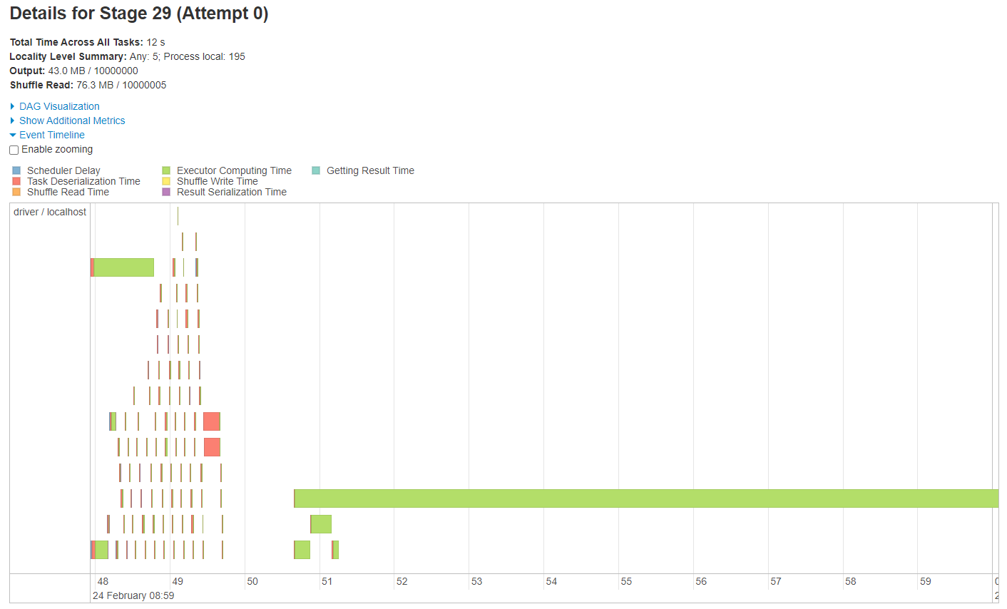
Fig. 24 Task timeline for skewed join

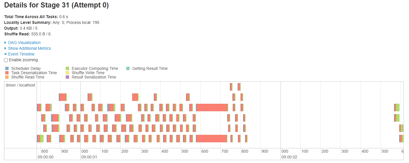
Fig. 25 Task timeline for skewed group by

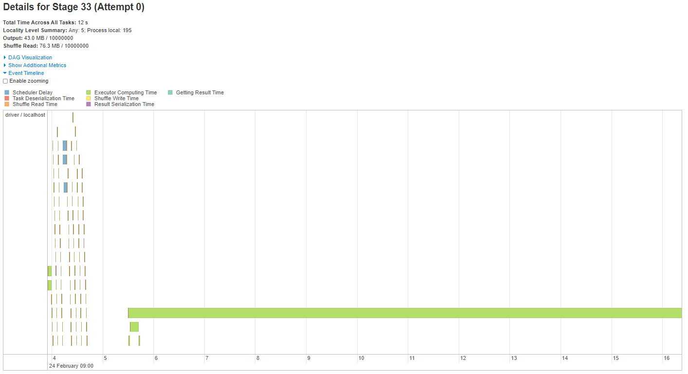
Fig. 26 Task timeline for skewed windows

It’s also useful to look at the Tasks table below the timeline to see how many records were processes in each of the 200 tasks. In the images below we have sorted the table by the Output Size / Records column (circled red) so that the largest tasks are at the top.

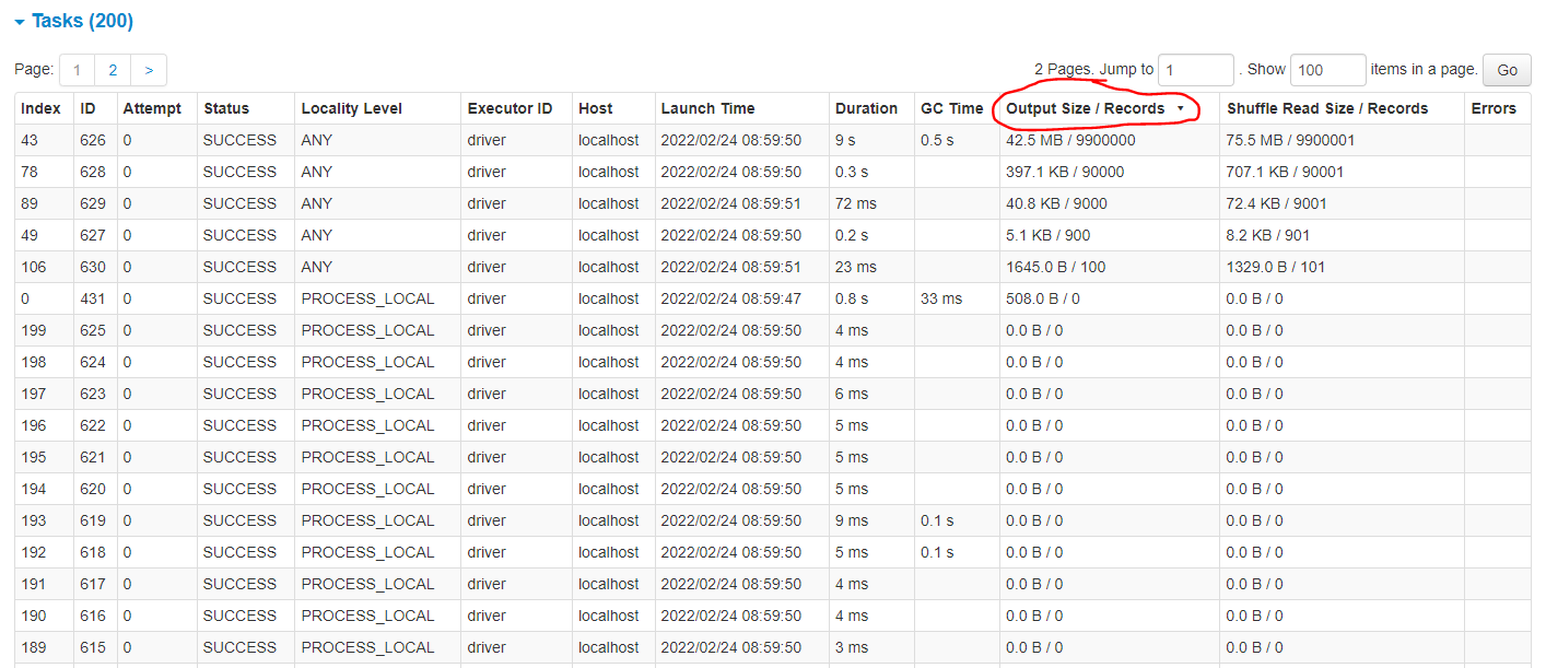
Fig. 27 Task details for skewed join

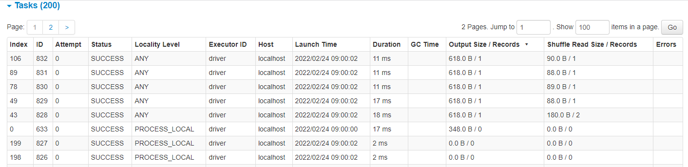
Fig. 28 Task details for skewed group by

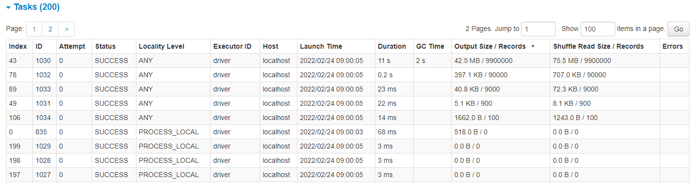
Fig. 29 Task details for skewed windows

One last piece of information we will gather is the partitioning information of the output DataFrames using the print_partitioning_info() function we defined above.

PythonR

print_partitioning_info(joined_df)

Python OutputR Output

+-------+-------+
|part_id|  count|
+-------+-------+
|     78|  90000|
|     43|9900000|
|     49|    900|
|    106|    100|
|     89|   9000|
+-------+-------+

Number of partitions: 200

PythonR

print_partitioning_info(grouped_df)

Python OutputR Output

+-------+-----+
|part_id|count|
+-------+-----+
|     78|    1|
|     43|    1|
|     49|    1|
|    106|    1|
|     89|    1|
+-------+-----+

Number of partitions: 200

PythonR

print_partitioning_info(window_df)

Python OutputR Output

+-------+-------+
|part_id|  count|
+-------+-------+
|      1|5000000|
|      0|5000000|
+-------+-------+

Number of partitions: 200

Discussion

Now that we have all the information on how Spark performed these processes we can compare the three cases.

All three operations involve an intermediate shuffle where the join key/grouped variable/windows are moved to the same partitions. This is called hashpartitioning() in the execution plan. As we mentioned previously, these are all wide transformations so the number of partitions of the output DataFrames are the same, 200. Listed below are the differences in processing and output DataFrames for the three operations.

Join

There was much more work to be done on the larger partition than the smaller ones. The Spark UI shows there were more records to process on the large partition therefore the task takes much longer. Note the number of records processed in each task matches the number of rows in each join key. The output DataFrame is partitioned by the join key.

Group by

In the case of the group by the skewed variable isn’t too much of an issue because the aggregation is quite simple and is optimised, therefore it is easy to process each partition whether there is skew or not. Again, the output DataFrame is partitioned by the grouped variable, this time there is one row on each partition.

Window

Like the join, there is more work to do on the larger partitions. However, unlike the join, the rows of the output DataFrame have the same partition IDs as the input DataFrame.

What does this mean in practice?

Highly skewed data is a common issue that causes slow processing with Spark. Above we have seen that skewed data causes skewed partitions when Spark processes wide transformations and can result in bottlenecks, where some tasks take much longer than others therefore not utilising the full potential of parallel processing. An even worse situation is where the skew causes spill, where the large partition cannot fit into its allocated memory on an executor and overflows temporarily onto disk. We cannot recreate the issue of spill in a local session but they are easy to spot in the Stage details page in the Spark UI.

This is where knowing your data can be useful. To help with the explanation we will refer to the join keys/groups/windows as groups. If a join/group by/window function is causing you issues, try to work out how many groups there are and the sizes of these groups. If there are lots on smaller groups it might help to increase spark.sql.shuffle.partitions and aim for greater parallel power with lots of smaller executors. If there are fewer groups you might want to scale more vertically so decrease spark.sql.shuffle.partitions and aim for a smaller number of bulkier executors.

If you are doing a join on a highly skewed DataFrame you might want to try a salted join. If you are dealing with skew in a window function you can apply a group by and join to achieve the same result. However, these are alternative solutions when dealing with highly skewed data and in most cases a regular join or window function are more efficient and makes the code more readable.

How should I partition my data?

The short answer is- don’t worry about it too much!

Let’s flip the question around. What are the consequences of getting the number of partitions “wrong”? Most of the time- nothing. You could spend hours trying to optimise the number of partitions and perhaps speed up the processing time to be twice as quick, but sometimes there are simpler things you can do that might speed up the processing by ten times or a hundred times the processing speed.

As the computer scientist Donald Knuth once wrote:

Premature optimization is the root of all evil (or at least most of it) in programming

-> Computer Programming as an Art (1974)

More importantly it’s good practice to be aware of the size of the DataFrame and the number of partitions as this will help to avoid obvious issues or over-partitioning, under-partitioning and highly skewed processes.

A more accurate answer depends on a variety of factors including: the size of the data, data types, distributions within the data, type of processing and other properties defined in the SparkSession. Here are some tips for quick wins:

• As suggested above, the first step is getting the code right. Only look to optimise if you’re running into performance issues.

• Decreasing the spark.sql.shuffle.partitions parameter is sensible for smaller datasets.

• If you search for an answer on the web, you might find the optimum size for a Spark partitions is 100-200MB. In practice, this is impossible to keep track of in an analysis script, but it gives you an idea of what is considered big or small.

• It makes sense for the number of partitions to be some multiple of the number of cores in the Spark session. This will help to avoid redundant cores.

Remember, it’s only worth experimenting on the optimum number if you have a real performance issue.

Partitions when Unioning or Binding DataFrames

You can append two DataFrames in PySpark that have the same schema with the .union() operation. In sparklyr, the equivalent operation is sdf_bind_rows() and R users will often refer to appending two DataFrames as binding.

The .union() function in PySpark and the sdf_bind_rows() function in sparklyr are both equivalent to UNION ALL in SQL. A regular UNION operation in SQL will remove duplicates, whereas .union() in PySpark and sdf_bind_rows() in sparklyr will not.

Unlike joining two DataFrames, .union()/sdf_bind_rows() does not involve a full shuffle, as the data does not move between partitions. Instead, the number of partitions in the unioned DataFrame is equal to the sum of the number of partitions in the two source DataFrames, i.e. if you union a DataFrame consisting of 100 partitions and one consisting of 50 partitions, your unioned DataFrame will have 150 partitions.

To avoid excessive number of partitions, you can use .coalesce() or .repartition() to reduce the number of partitions (use sdf_coalesce() or sdf_repartition() in sparklyr). The DataFrame will also get repartitioned when a wide transformation is applied to the DataFrame (also called a shuffle), e.g. with a .groupBy() or .orderBy().

It is also worth being aware that storing data on HDFS as many small files is inefficient, both in terms of how the data is stored and in reading it in. Unioning many DataFrames and then writing straight to HDFS can be a cause of this issue. For more information on the small file issue, see the previous section on Partition sizes.

First we will stop the previous spark sessions and start a new Spark session which limits the number of partitions to 12, read the Animal Rescue data, group by animal and year, and then count. The grouping and aggregation will cause a shuffle, meaning that the DataFrame will have 12 partitions, as we set spark.sql.shuffle.partitions to 12 in the SparkSession.builder.

PythonR

from pyspark.sql import SparkSession, functions as F

# Stop previous spark session and create new spark session

spark.stop()

spark = (SparkSession.builder.master("local[2]")
         .appName("partitions")
         .config("spark.sql.shuffle.partitions", 12)
         .getOrCreate())


rescue_path_csv = config["rescue_path_csv"]

# # Read in and shuffle data
rescue = (spark.read.csv(rescue_path_csv, header=True, inferSchema=True)  
          .withColumnRenamed("IncidentNumber", "incident_number")
          .withColumnRenamed("AnimalGroupParent", "animal_group")
          .withColumnRenamed("CalYear", "cal_year")
          .groupBy("animal_group", "cal_year")
          .agg(F.count("incident_number").alias("animal_count")))

rescue.limit(5).toPandas()

Python OutputR Output

                       animal_group  cal_year  animal_count
0                              Bird      2010            99
1                           Hamster      2011             3
2  Unknown - Domestic Animal Or Pet      2012            18
3  Unknown - Heavy Livestock Animal      2012             4
4                             Sheep      2012             1

We can confirm the number of partitions of the rescue DataFrame using .rdd.getNumPartitions():

PythonR

print('Rescue partitions:',rescue.rdd.getNumPartitions())

Python OutputR Output

Rescue partitions: 12

Now create will create some smaller DataFrames, containing different animals, by filtering the rescue data. We will preview just the dogs data, as all others will be of a similar format:

PythonR

dogs = rescue.filter(F.col("animal_group") == "Dog")
cats = rescue.filter(F.col("animal_group") == "Cat")
hamsters = rescue.filter(F.col("animal_group") == "Hamster")

dogs.limit(5).toPandas()

Python OutputR Output

  animal_group  cal_year  animal_count
0          Dog      2011           103
1          Dog      2017            81
2          Dog      2009           132
3          Dog      2012           100
4          Dog      2014            90

We can check that each of these DataFrames has 12 partitions:

PythonR

print(' Dog partitions:', dogs.rdd.getNumPartitions(),
      '\n Cat partitions:', cats.rdd.getNumPartitions(),
      '\n Hamster partitions:', hamsters.rdd.getNumPartitions())

Python OutputR Output

 Dog partitions: 12 
 Cat partitions: 12 
 Hamster partitions: 12

When we apply the union function, the number of partitions in the unioned DataFrame will be the sum of partitions in each DataFrame. In this case we will now have 12 + 12 = 24 partitions:

PythonR

dogs_and_cats = dogs.union(cats)
print('Dogs and Cats union partitions:',dogs_and_cats.rdd.getNumPartitions())

Python OutputR Output

Dogs and Cats union partitions: 24

Unioning another DataFrame adds another 12 partitions to make 36 (24 + 12):

PythonR

dogs_cats_and_hamsters = dogs_and_cats.union(hamsters)
print('Dogs, Cats and Hamsters union partitions:',dogs_cats_and_hamsters.rdd.getNumPartitions())

Python OutputR Output

Dogs, Cats and Hamsters union partitions: 36

Although we only have 36 partitions here it is easy to see how this might get excessive with too many .union() statements. This can also become a bigger problem if the number of partitons is left to its default value of 200, where we would end up with 600 partitions!

A subsequent shuffle (e.g. sorting the DataFrame) will reset the number of partitions to that specified in spark.sql.shuffle.partitions:

PythonR

dogs_cats_and_hamsters.orderBy("animal_group", "cal_year").rdd.getNumPartitions()

Python OutputR Output

12

You can also use .repartition() or .coalesce(). .repartition() involves a shuffle of the DataFrame and puts the data into roughly equal partition sizes, whereas .coalesce() combines partitions without a full shuffle, and so is more efficient, although at the potential cost of less equal partition sizes and therefore potential skew in the data. For more information see the previous section on Partition sizes.

PythonR

dogs_cats_and_hamsters.repartition(20).rdd.getNumPartitions()

Python OutputR Output

20

Further information on managing partitions while writing data can now be found in the Reading and Writing Data in Spark page.

Further resources

Spark at the ONS Articles:

• Spark Application and UI

• Shuffling

• Guidance on Spark Sessions

• Window Functions in Spark

• Salted Joins

• Checkpoint and Staging Tables

• Reading and Writing Data in Spark

PySpark Documentation:

• .coalesce()

• SparkSession

• .getNumPartitions()

• .repartition()

• .coalesce()

• .rdd.mapPartitions()

• DataFrameWriter.partitionBy()

• .union()

Python Documentation:

• subprocess

sparklyr and tidyverse Documentation:

• sdf_coalesce()

• sdf_repartition()

• sdf_num_partitions()

• spark_apply()

• sdf_bind_rows()

Spark Documentation:

• Spark Configuration:

  • Execution Behaviour

  • Runtime SQL Configuration

• round

• bround