Caching

Caching Spark DataFrames can be useful for two reasons:

1. To estimate the size of a DataFrame and its partitions in memory

2. Improve Spark performance by breaking the lineage of a DataFrame

In this article we will firstly introduce caching to estimate the size of a DataFrame then see an example of where caching is useful to remove repeated runs of an execution plan.

For a more detailed discussion on persistence in Spark please see the Persisting article.

How big is my DataFrame?

A simple use of persistence in Spark is to find out how much memory is used to store a DataFrame. This is a tricky subject because the amount of memory or disk space a data set uses depends on many factors, including:

1. whether the data are on disk (in storage) or in memory (being used)

2. format (e.g. csv or parquet on disk, pandas or Spark DataFrame in memory)

3. data types

4. type of serialisation (compression)

Most of this list is beyond the scope of this article, but it’s useful to know that these factors effect the exact size of a data set.

As usual we’ll start with some imports and creating a Spark session.

PythonR

from pyspark.sql import SparkSession, functions as F
import yaml

spark = (SparkSession.builder.master("local[2]")
         .appName("cache")
         .getOrCreate())

Next we need some data. Here we’re using a small amount of data because we’re running a local session which has very limited resource.

Note that .cache() in PySpark is a transformation, so to initiate moving the data into memory we need an action, hence the .count().

In sparklyr there is a force=TRUE argument in the tbl_cache() function meaning there is no need to pipe this into a row count. Also note that the name of the DataFrame will appear in the Spark UI, which is a nice feature in sparklyr. To do the same in PySpark we would need to register the DataFrame as a temporary table and give it a name.

PythonR

with open("../../../config.yaml") as f:
    config = yaml.safe_load(f)

population = spark.read.parquet(config['population_path'])

population.cache().count()

Python Output

2297

Now we can take a look in the Spark UI, which is reached using the URL http://localhost:4040/jobs/. Note this address is used for a local Spark session, for more information on how to navigate to the Spark UI see the documentation on monitoring.

Within the Spark UI, if you were to head over to the Storage tab you would see an RDD stored in memory, in two partitions and using 35.7 KB of executor memory. More on RDDs in the Shuffling article.

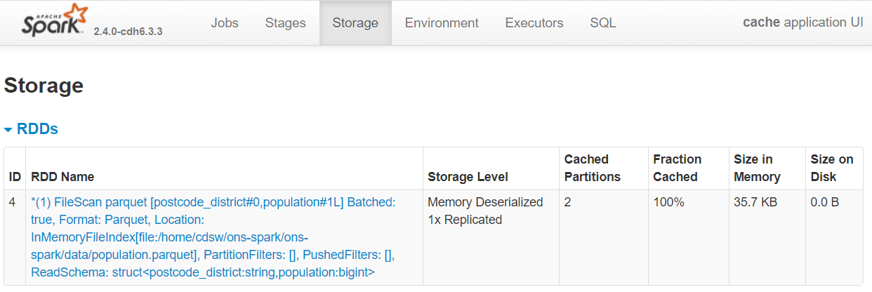
Fig. 30 DataFrame cached in memory

You can also click on the RDD name to get more information, such as how many executors are being used and the size of each partition.

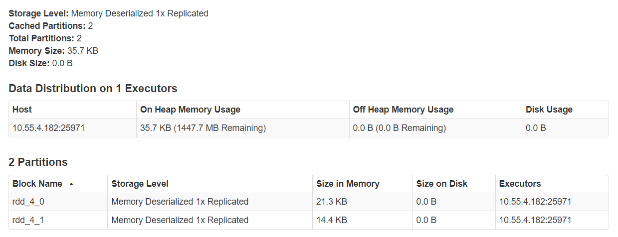
Fig. 31 Cache details

Persist

There is another function that can be used to persist DataFrames, .persist()/sdf_persist() in PySpark/sparklyr. This is a general form of .cache()/tbl_cache(). It is similar to doing a cache but we are able to specify where to store the data, e.g. use memory but allow spill over to executor disk if the executor memory is full. .persist()/sdf_persist() takes a StorageLevel argument to specify where to cache the data. Options for storage levels are:

• MEMORY_ONLY

• MEMORY_AND_DISK

• MEMORY_ONLY_SER

• MEMORY_AND_DISK_SER

• DISK_ONLY

• OFF_HEAP

Using the MEMORY_ONLY option is equivalent to .cache()/tbl_cache(). More information on storage levels can be found in the Apache Spark documentation. The only detail we will add here is that DISK in this instance refers to the executor disk and not the file system.

There’s an example below to see how this is used, first we will unpersist the previous DataFrame so that we don’t fill our cache memory with unused data. Note this time in sparklyr we need to add a row count.

PythonR

population.unpersist()

Python Output

DataFrame[postcode_district: string, population: bigint]

PythonR

from pyspark import StorageLevel
population.persist(StorageLevel.DISK_ONLY).count()

Python OutputR Output

2297

Before we move on, head back to the Spark UI and have a look at how much space the population DataFrame uses on disk.

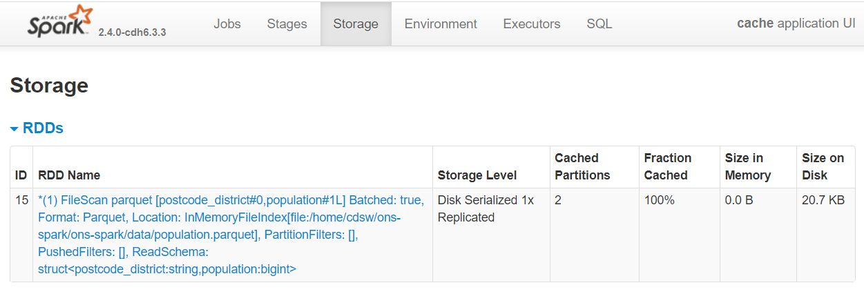
Fig. 32 DataFrame cached on disk

Is this what you expected? Why is this number different to persisting in memory? Because there is some compression involved in data written on disk.

Databricks, a company founded by the creators of Apache Spark, suggest the use cases for .persist()/sdf_persist() are rare. The are often cases where you might want to persist using cache()/tbl_cache(), write to disk, use .checkpoint()/sdf_checkpoint() or staging tables, but the options that .persist()/sdf_persist() present are not as useful. For a more detailed discussion about these options see the Persisting article.

PythonR

population.unpersist()

Python Output

DataFrame[postcode_district: string, population: bigint]

Using cache for more efficient coding

Let’s take a look at caching to speed up some processing. The scenario is that we want to read in some data and apply some cleaning and preprocessing. Then using this cleansed DataFrame we want to produce three tables as outputs for a publication.

The data we will use are the animal rescue data set collected by the London Fire Brigade.

Preparing the data

PythonR

rescue = spark.read.csv(
    config['rescue_path_csv'], 
    header=True, inferSchema=True, 
)

The DataFrame is read into a single partition, which is fine because it’s a small amount of data. However, we’ll repartition to later demonstrate a feature of Spark.

PythonR

rescue = rescue.repartition(2)

rescue = rescue.drop(
    'WardCode', 
    'BoroughCode', 
    'Easting_m', 
    'Northing_m', 
    'Easting_rounded', 
    'Northing_rounded'
)


rescue = (rescue
          .withColumnRenamed("PumpCount", "EngineCount")
          .withColumnRenamed("FinalDescription", "Description")
          .withColumnRenamed("HourlyNotionalCost(£)", "HourlyCost")
          .withColumnRenamed("IncidentNotionalCost(£)", "TotalCost")
          .withColumnRenamed("OriginofCall", "OriginOfCall")
          .withColumnRenamed("PumpHoursTotal", "JobHours")
          .withColumnRenamed("AnimalGroupParent", "AnimalGroup")
)


rescue = rescue.withColumn(
    "DateTimeOfCall", F.to_date(rescue.DateTimeOfCall, "dd/MM/yyyy")
)


rescue = rescue.withColumn(
    "IncidentDuration", 
    rescue.JobHours / rescue.EngineCount
)


rescue = rescue.na.drop(subset=["TotalCost", "IncidentDuration"])

Note that the above cells executed very quickly. Remember this is because they’re all transformations, which means Spark hasn’t executed the code yet; take a look at the Spark UI if you need convincing. So far Spark has created an execution plan but is waiting for an action to implement the plan.

Analysis

Now we have our cleansed DataFrame we can go on to produce some tables for our article on animal rescue costs for the London Fire Brigade. Here we will put the code into functions because we will rerun these snippets of code multiple times in this notebook.

PythonR

def get_top_10_incidents(sdf):
    return (sdf
        .select("CalYear", "PostcodeDistrict", "AnimalGroup", "IncidentDuration", "TotalCost")
        .sort("TotalCost", ascending=False)
        .limit(10)
    )

def get_mean_cost_by_animal(sdf):
    return (sdf
        .groupBy("AnimalGroup")
        .agg(F.mean("TotalCost").alias('MeanCost'))
        .sort("MeanCost", ascending=False)
        .limit(10)
    )

def get_summary_cost_by_animal(sdf):
    return (sdf.filter(
                rescue.AnimalGroup.isin(
                    "Goat", 
                    "Bull", 
                    "Fish", 
                    "Horse")
            )
            .groupBy("AnimalGroup")
            .agg(
                F.min('TotalCost').alias('Min'), 
                F.avg('TotalCost').alias('Mean'), 
                F.max('TotalCost').alias('Max'), 
                F.count('TotalCost').alias('Count'))
            .sort("Mean", ascending=False)
    )

Next we will call the above functions and show the results

PythonR

top_10_incidents = get_top_10_incidents(rescue)
top_10_incidents.show(truncate=False)

Python OutputR Output

+-------+----------------+---------------------+----------------+---------+
|CalYear|PostcodeDistrict|AnimalGroup          |IncidentDuration|TotalCost|
+-------+----------------+---------------------+----------------+---------+
|2016   |NW5             |Cat                  |4.0             |3912.0   |
|2013   |E4              |Horse                |6.0             |3480.0   |
|2015   |TN14            |Horse                |5.0             |2980.0   |
|2018   |UB4             |Horse                |4.0             |2664.0   |
|2014   |TW4             |Cat                  |4.5             |2655.0   |
|2011   |E17             |Horse                |3.0             |2340.0   |
|2011   |E14             |Deer                 |3.0             |2340.0   |
|2011   |E17             |Horse                |3.0             |2340.0   |
|2018   |TN16            |Unknown - Wild Animal|3.5             |2296.0   |
|2017   |N19             |Cat                  |3.5             |2282.0   |
+-------+----------------+---------------------+----------------+---------+

PythonR

mean_cost_by_animal = get_mean_cost_by_animal(rescue)
mean_cost_by_animal.show(truncate=False)

Python OutputR Output

+------------------------------------------------+------------------+
|AnimalGroup                                     |MeanCost          |
+------------------------------------------------+------------------+
|Goat                                            |1180.0            |
|Bull                                            |780.0             |
|Fish                                            |780.0             |
|Horse                                           |747.4350649350649 |
|Unknown - Animal rescue from water - Farm animal|709.6666666666666 |
|Cow                                             |624.1666666666666 |
|Hedgehog                                        |520.0             |
|Lamb                                            |520.0             |
|Deer                                            |423.8829787234043 |
|Unknown - Wild Animal                           |390.03636363636366|
+------------------------------------------------+------------------+

PythonR

summary_cost_by_animal = get_summary_cost_by_animal(rescue)
summary_cost_by_animal.show()

Python OutputR Output

+-----------+------+-----------------+------+-----+
|AnimalGroup|   Min|             Mean|   Max|Count|
+-----------+------+-----------------+------+-----+
|       Goat|1180.0|           1180.0|1180.0|    1|
|       Bull| 780.0|            780.0| 780.0|    1|
|       Fish| 260.0|            780.0|1300.0|    2|
|      Horse| 255.0|747.4350649350649|3480.0|  154|
+-----------+------+-----------------+------+-----+

Great- we have our tables. Let’s take a look at the individual steps Spark carried out to create our outputs.

Investigate the Spark UI

Go into the Spark UI and look at the SQL tab which lists the queries that are created from our PySpark code. Alternatively, we could use the Jobs tab, but the SQL tab has more detailed information for our needs here.

Click on the query with a description that starts with ‘csv’ and look at the DAG diagram. DAG stands for Directed Acyclic Graph and is often used to describe a process.

Fig. 33 File scan to infer DataFrame schema

This query is glancing at the animal_rescue.csv file to get the schema so that following transformations can be validated before being added to the execution plan (it does this because we asked Spark to infer the schema). Doing this for large files can take several minutes, so for large data sets use parquet files or Hive tables, which store the schema for you.

The next three queries (highlighted below) are the functions we have called above. Look at the DAG for each query by clicking on the descriptions, what are your observations?

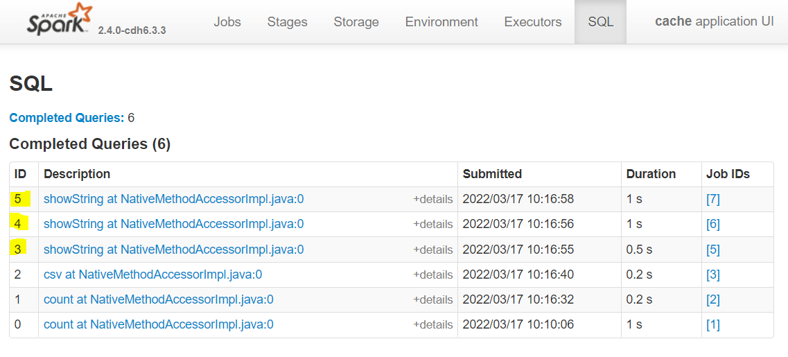
Fig. 34 Analysis duration without cache

Observations

• Spark has changed the order of our transformations. We’ll look at this later.

• It’s difficult to make sense of some boxes.

• Every single one starts with reading in the data (Scan csv).

The last point above means that Spark is reading in the file at the beginning of the job, and assuming there are no skipped stages, Spark is repeating the cleaning process for each output table.

Using a cache

What we need to do is to persist the rescue DataFrame so when we start our analysis functions Spark will use the cleansed and persisted DataFrame as the starting point.

Let’s cache the rescue DataFrame.

PythonR

rescue.cache().count()

Python Output

5860

PythonR

get_top_10_incidents(rescue).show()

Python OutputR Output

+-------+----------------+--------------------+----------------+---------+
|CalYear|PostcodeDistrict|         AnimalGroup|IncidentDuration|TotalCost|
+-------+----------------+--------------------+----------------+---------+
|   2016|             NW5|                 Cat|             4.0|   3912.0|
|   2013|              E4|               Horse|             6.0|   3480.0|
|   2015|            TN14|               Horse|             5.0|   2980.0|
|   2018|             UB4|               Horse|             4.0|   2664.0|
|   2014|             TW4|                 Cat|             4.5|   2655.0|
|   2011|             E14|                Deer|             3.0|   2340.0|
|   2011|             E17|               Horse|             3.0|   2340.0|
|   2011|             E17|               Horse|             3.0|   2340.0|
|   2018|            TN16|Unknown - Wild An...|             3.5|   2296.0|
|   2017|             N19|                 Cat|             3.5|   2282.0|
+-------+----------------+--------------------+----------------+---------+

PythonR

get_mean_cost_by_animal(rescue).show()

Python OutputR Output

+--------------------+------------------+
|         AnimalGroup|          MeanCost|
+--------------------+------------------+
|                Goat|            1180.0|
|                Bull|             780.0|
|                Fish|             780.0|
|               Horse| 747.4350649350649|
|Unknown - Animal ...| 709.6666666666666|
|                 Cow| 624.1666666666666|
|            Hedgehog|             520.0|
|                Lamb|             520.0|
|                Deer| 423.8829787234043|
|Unknown - Wild An...|390.03636363636366|
+--------------------+------------------+

PythonR

get_summary_cost_by_animal(rescue).show()

Python OutputR Output

+-----------+------+-----------------+------+-----+
|AnimalGroup|   Min|             Mean|   Max|Count|
+-----------+------+-----------------+------+-----+
|       Goat|1180.0|           1180.0|1180.0|    1|
|       Fish| 260.0|            780.0|1300.0|    2|
|       Bull| 780.0|            780.0| 780.0|    1|
|      Horse| 255.0|747.4350649350649|3480.0|  154|
+-----------+------+-----------------+------+-----+

Look at the Spark UI. Below is the DAG for the latest query.

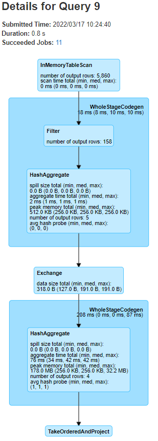
Fig. 35 SQL DAG using cached DataFrame

This time Spark didn’t read in the data from disk and apply the cleaning, we have broken the lineage. We know this because the DAG starts with a InMemoryTableScan, i.e. the cache. Note that this diagram consists of fewer stages than we had previously. Another sign of cached data being used is the presence of Skipped Stages on the Jobs page.

The important point here is that we were doing repeated computations on a DataFrame, i.e. aggregations on the cleansed data. When this happens it may well be more efficient to persist the data before the repeated calculations. We should check this for our case.

There are many factors that contribute towards the time taken for each query that make benchmarking in Spark complex. When running the source notebook, sometimes the processing will be faster after the cache, but sometimes it will be slower. If we run the last three code cells above once more and look at the times we see that the processing after the cache was generally quicker.

Each function is labelled in the image below. The first run was without caching, the second was with caching and the third was a second run with cached data.

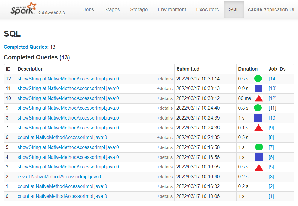
Fig. 36 Processing time without and with cache

Further Resources

Spark at the ONS Articles:

• Persisting

• Shuffling:

  • A Quick Note on RDDs

• Spark Application and UI

PySpark Documentation:

• .count()

• .cache()

• .persist()

• .checkpoint()

sparklyr and tidyverse Documentation:

• tbl_cache()

• sdf_persist()

• sdf_checkpoint()

Spark Documentation:

• Monitoring and Instrumentation

• RDD Persistence

Other Links:

• Databricks